Last updated: 2024-01-31

Checks: 6 1

Knit directory: SuperCellCyto-analysis/

This reproducible R Markdown analysis was created with workflowr (version 1.7.0). The Checks tab describes the reproducibility checks that were applied when the results were created. The Past versions tab lists the development history.

R Markdown file: uncommitted changes

The R Markdown file has unstaged changes. To know which version of the R Markdown file created these results, you’ll want to first commit it to the Git repo. If you’re still working on the analysis, you can ignore this warning. When you’re finished, you can run wflow_publish to commit the R Markdown file and build the HTML.

Environment: empty

Great job! The global environment was empty. Objects defined in the global environment can affect the analysis in your R Markdown file in unknown ways. For reproduciblity it’s best to always run the code in an empty environment.

Seed: set.seed(42)

The command set.seed(42) was run prior to running the code in the R Markdown file. Setting a seed ensures that any results that rely on randomness, e.g. subsampling or permutations, are reproducible.

Session information: recorded

Great job! Recording the operating system, R version, and package versions is critical for reproducibility.

Cache: none

Nice! There were no cached chunks for this analysis, so you can be confident that you successfully produced the results during this run.

File paths: relative

Great job! Using relative paths to the files within your workflowr project makes it easier to run your code on other machines.

Repository version: 264aa64

Great! You are using Git for version control. Tracking code development and connecting the code version to the results is critical for reproducibility.

The results in this page were generated with repository version 264aa64. See the Past versions tab to see a history of the changes made to the R Markdown and HTML files.

Note that you need to be careful to ensure that all relevant files for the analysis have been committed to Git prior to generating the results (you can use wflow_publish or wflow_git_commit). workflowr only checks the R Markdown file, but you know if there are other scripts or data files that it depends on. Below is the status of the Git repository when the results were generated:


Ignored files:
    Ignored:    .DS_Store
    Ignored:    .Rhistory
    Ignored:    .Rproj.user/
    Ignored:    analysis/.DS_Store
    Ignored:    code/.DS_Store
    Ignored:    code/b_cell_identification/.DS_Store
    Ignored:    code/b_cell_identification/runtime_benchmark/.DS_Store
    Ignored:    code/batch_correction/.DS_Store
    Ignored:    code/batch_correction/runtime_benchmark/.DS_Store
    Ignored:    code/explore_supercell_purity_clustering/.DS_Store
    Ignored:    code/explore_supercell_purity_clustering/functions/.DS_Store
    Ignored:    code/explore_supercell_purity_clustering/louvain_all_cells/.DS_Store
    Ignored:    code/explore_supercell_purity_clustering/louvain_all_cells/levine_32dim/.DS_Store
    Ignored:    code/label_transfer/.Rhistory
    Ignored:    data/.DS_Store
    Ignored:    data/bodenmiller_cytof/
    Ignored:    data/explore_supercell_purity_clustering/
    Ignored:    data/haas_bm/
    Ignored:    data/oetjen_bm_dataset/
    Ignored:    data/trussart_cytofruv/
    Ignored:    output/.DS_Store
    Ignored:    output/bodenmiller_cytof/
    Ignored:    output/explore_supercell_purity_clustering/
    Ignored:    output/label_transfer/
    Ignored:    output/oetjen_b_cell_panel/
    Ignored:    output/trussart_cytofruv/

Untracked files:
    Untracked:  code/b_cell_identification/additional_code/
    Untracked:  code/batch_correction/additional_code/
    Untracked:  code/explore_supercell_purity_clustering/additional_code/
    Untracked:  code/label_transfer/additional_code/

Unstaged changes:
    Modified:   SuperCellCyto-analysis.Rproj
    Modified:   analysis/b_cells_identification.Rmd
    Modified:   analysis/batch_correction.Rmd
    Modified:   analysis/explore_supercell_purity_clustering.Rmd

Note that any generated files, e.g. HTML, png, CSS, etc., are not included in this status report because it is ok for generated content to have uncommitted changes.

These are the previous versions of the repository in which changes were made to the R Markdown (analysis/explore_supercell_purity_clustering.Rmd) and HTML (docs/explore_supercell_purity_clustering.html) files. If you’ve configured a remote Git repository (see ?wflow_git_remote), click on the hyperlinks in the table below to view the files as they were in that past version.

File	Version	Author	Date	Message
html	98e46e0	Givanna Putri	2023-08-15	Build site.
html	a55c3ba	Givanna Putri	2023-07-28	Build site.
html	366514e	Givanna Putri	2023-07-28	Build site.
Rmd	402358b	Givanna Putri	2023-07-28	wflow_publish(c("analysis/*Rmd"))

Introduction

We assessed whether supercells could preserve the biological diversity inherent in a dataset, and whether the clustering of supercells could expedite the process of cell type identification without compromising accuracy.

Datasets

We ran SuperCellCyto on two publicly accessible cytometry datasets from Weber and Robinson’s clustering benchmarking study (Weber and Robinson 2016).

The cell type annotation were done using manual gating by an immunologist.

Levine_32dim dataset (Levine et al. 2015) measures the expression of 32 markers in bone marrow cells from healthy human donors, comprised of 2 samples, 265,627 cells, and 14 cell types, with cell type labels assigned to 39% (104,184) of cells.
Samusik_all dataset (Samusik et al. 2016) quantifies the expression of 39 markers in bone marrow cells from healthy mice. There are 10 samples, 841,644 cells, and 24 cell types, with cell type labels assigned to 61% (514,386) of cells.

The R scripts required to run SuperCellCyto and perform clustering can be found in the code/explore_supercell_purity_clustering directory.

Load libraries and data

library(data.table)
library(ggplot2)
library(scales)
library(here)
library(stringr)
library(ggridges)
library(viridis)

levine_res_dir <- here("output", "explore_supercell_purity_clustering",
                       "20230511", "levine_32dim")
samusik_res_dir <- here("output", "explore_supercell_purity_clustering",
                        "20230511", "samusik_all")

Data Reduction Amount

How many supercells were generated per gamma value?

gamma <- seq(5, 50, 5)
n_supercells_levine <- sapply(gamma, function(gam) {
  nrow(fread(here(levine_res_dir, "supercell_runs",
                  paste0("supercellExpMat_gamma", gam, ".csv"))))
})
n_supercells_samusik <- sapply(gamma, function(gam) {
  nrow(fread(here(samusik_res_dir, "supercell_runs",
                  paste0("supercellExpMat_gamma", gam, ".csv"))))
})

n_cells_levine <- nrow(fread(here(levine_res_dir, "supercell_runs",
                                  "supercellCellMap_gamma5.csv")))
n_cells_samusik <- nrow(fread(here(samusik_res_dir, "supercell_runs",
                                   "supercellCellMap_gamma5.csv")))

n_supercells <- data.table(gamma, n_supercells_levine, n_supercells_samusik)
n_supercells

    gamma n_supercells_levine n_supercells_samusik
 1:     5               53125               168328
 2:    10               26563                84164
 3:    15               17709                56109
 4:    20               13282                42082
 5:    25               10625                33666
 6:    30                8854                28055
 7:    35                7589                24048
 8:    40                6641                21042
 9:    45                5903                18702
10:    50                5313                16832

n_supercells_plot <- data.table(
  gamma = rep(gamma, 2),
  n_cells = c(n_supercells_levine, n_supercells_samusik),
  dataset = c(rep("Levine_32dim", length(gamma)),
              rep("Samusik_all", length(gamma)))
)
n_supercells_plot$gamma <- factor(n_supercells_plot$gamma, levels = c(gamma))
n_supercells_plot <- n_supercells_plot[order(gamma)]

facet_labels <- c(
  "Levine_32dim" = paste0("Levine_32dim\n",
                          format(n_cells_levine, big.mark = ","),
                          " cells"),
  "Samusik_all" = paste0("Samusik_all\n",
                         format(n_cells_samusik, big.mark = ","),
                         " cells")
)
ggplot(n_supercells_plot, aes(x = gamma, y = n_cells)) +
  geom_bar(stat = "identity", fill = "blue") +
  facet_wrap(~dataset, labeller = labeller(dataset = facet_labels)) +
  scale_y_continuous(labels = label_comma(), breaks = pretty_breaks(n = 10)) +
  labs(
    y = "Number of supercells", x = "Gamma",
    title = "Number of supercells generated per gamma value"
  ) +
  theme_bw()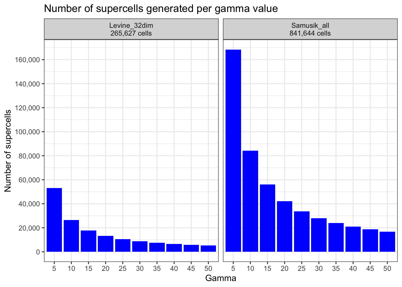

Version	Author	Date
366514e	Givanna Putri	2023-07-28

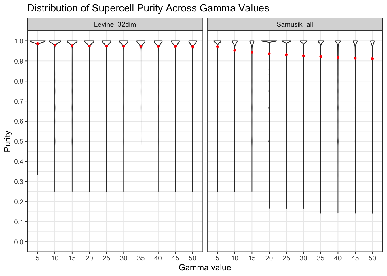
Impact of gamma parameters on Supercell Purity

We investigate how gamma parameters influence Supercell Purity. Gamma values determine the granularity of the Supercell with a direct relationship: gamma = number of cells / number of supercells. A larger gamma implies fewer, larger supercells (each supercell capturing more cells), while a smaller gamma leads to more, smaller supercells.

levine_purity <- fread(here(levine_res_dir, "evaluation",
                            "supercell_purities.csv"))
levine_purity[, data_source := "Levine_32dim"]
samusik_purity <- fread(here(samusik_res_dir, "evaluation",
                             "supercell_purities.csv"))
samusik_purity[, data_source := "Samusik_all"]
purity_scores <- rbind(levine_purity, samusik_purity)
purity_scores[, gamma := factor(gamma)]

ggplot(purity_scores, aes(y = purity, x = gamma)) +
  geom_violin() +
  stat_summary(fun = mean, geom = "point", color = "red", size = 1) +
  facet_wrap(~data_source) +
  theme_bw() +
  scale_y_continuous(breaks = pretty_breaks(n = 10), limits = c(0, 1)) +
  labs(
    y = "Purity", x = "Gamma value",
    title = "Distribution of Supercell Purity Across Gamma Values"
  )

Version	Author	Date
366514e	Givanna Putri	2023-07-28

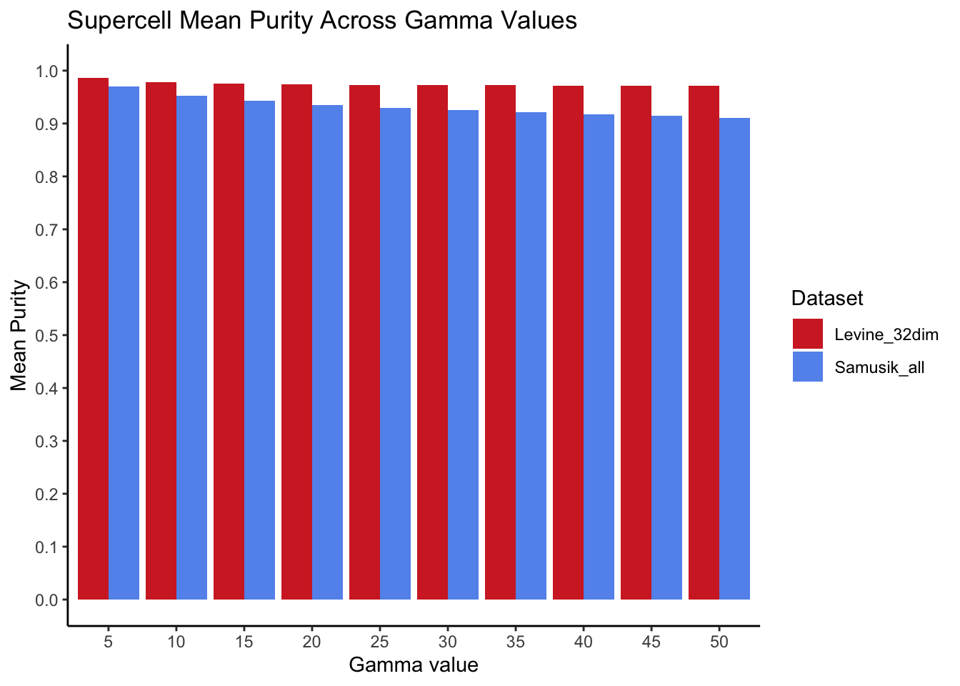
What are the mean purity scores?

mean_purity <- purity_scores[, .(mean_purity = mean(purity)), by = c("gamma", "data_source")]

ggplot(mean_purity, aes(x = gamma, y = mean_purity, fill = data_source)) +
  geom_bar(stat = "identity", position = position_dodge()) +
  scale_fill_manual(values = c("Levine_32dim" = "#D22B2B", "Samusik_all" = "#6495ED")) +
  scale_y_continuous(breaks = pretty_breaks(n = 10), limits = c(0, 1)) +
  theme_classic() +
  labs(
    x = "Gamma value", y = "Mean Purity", fill = "Dataset",
    title = "Supercell Mean Purity Across Gamma Values"
  )

Version	Author	Date
366514e	Givanna Putri	2023-07-28

Proportion of purity scores < 0.5 across all gamma values?

poor_purity <- purity_scores[purity < 0.5, ]
poor_purity_cnt <- merge.data.table(
  poor_purity[, .N, by = "data_source"],
  purity_scores[, .N, by = "data_source"],
  by = "data_source",
  suffixes = c("_poor", "_all")
)
poor_purity_cnt[, percent := N_poor * 100 / N_all]

poor_purity_cnt

    data_source N_poor  N_all    percent
1: Levine_32dim     56 149116 0.03755466
2:  Samusik_all   2572 432821 0.59424104

For both datasets, we observed very high mean purity scores across all gamma values (purity > 0.9), with the vast proportion of supercells attaining a purity score of 1. A small percentage of supercells (0.04% for Levine_32dim and 0.59% for Samusik_all) obtained purity < 0.5.

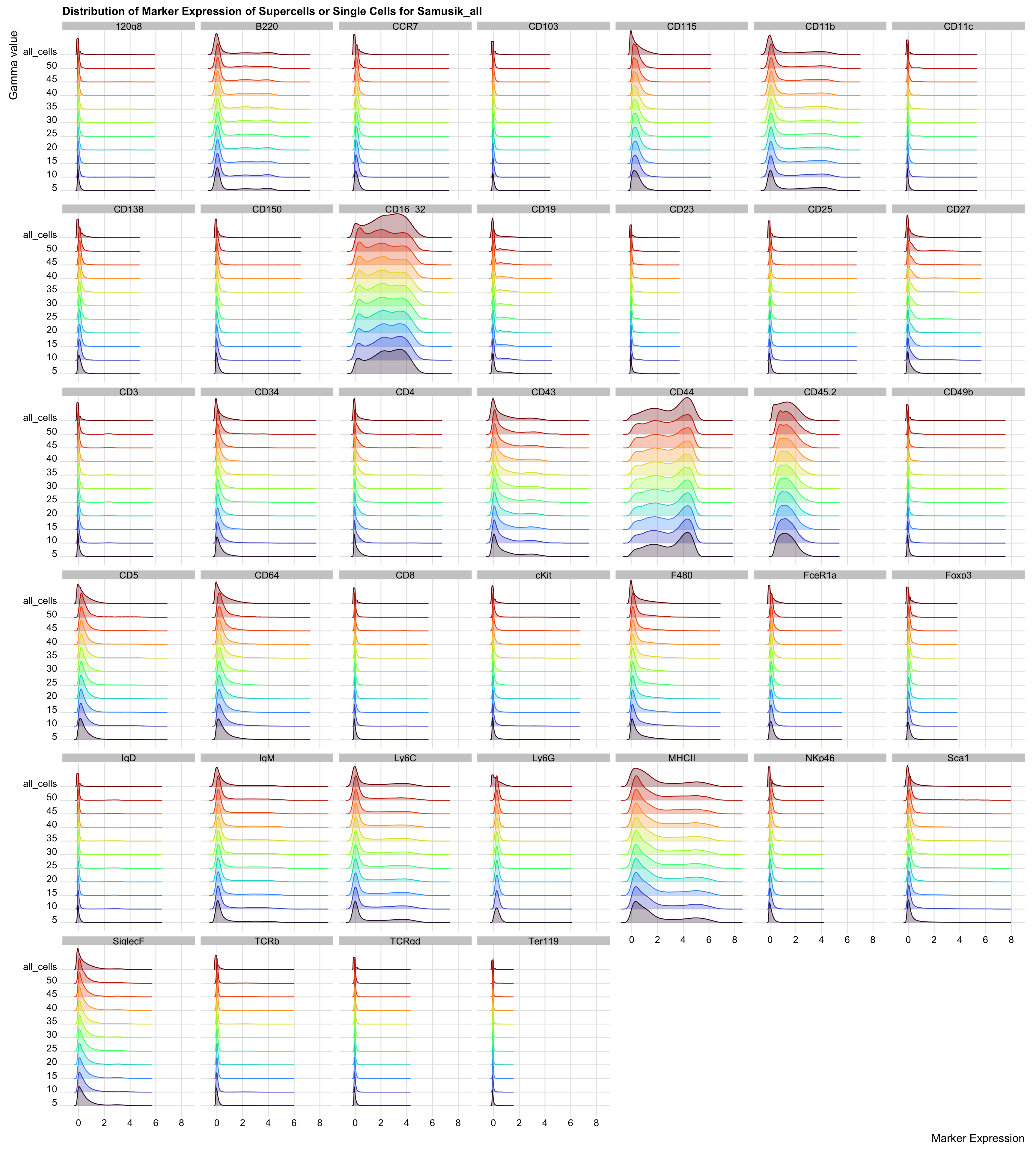
Comparing Marker Expression Distribution

Samusik data

markers <- fread(here(
  "data", "explore_supercell_purity_clustering",
  "samusik_all", "samusik_all_asinh_markers_info.csv"
))
markers <- markers[marker_class != "none"]

raw_dat <- fread(here(
  "data", "explore_supercell_purity_clustering",
  "samusik_all", "samusik_all_asinh.csv"
))
raw_dat$from <- "all_cells"


supercell_dat <- rbindlist(lapply(seq(5, 50, by = 5), function(gamma_val) {
  dt <- fread(here(
    samusik_res_dir, "supercell_runs",
    paste0("supercellExpMat_gamma", gamma_val, ".csv")
  ))
  dt$from <- gamma_val
  return(dt[, c("from", paste0(markers$marker_name, "_asinh_cf5")), with = FALSE])
}))

all_dat <- rbind(supercell_dat,
                 raw_dat[, c("from", paste0(markers$marker_name, "_asinh_cf5")), with = FALSE])
all_dat$from <- factor(all_dat$from, levels = c(seq(5, 50, 5), "all_cells"))

all_dat_molten <- melt(all_dat, id.vars = "from")
all_dat_molten[, variable := gsub("_asinh_cf5", "", variable)]

ggplot(all_dat_molten, aes(x = value, y = from, colour = from, fill = from)) +
  geom_density_ridges(alpha = 0.3) +
  scale_colour_viridis(option = "turbo", discrete = TRUE, guide = "none") +
  scale_fill_viridis(option = "turbo", discrete = TRUE, guide = "none") +
  theme_ridges() +
  facet_wrap(~variable) +
  scale_x_continuous(breaks = pretty_breaks(n = 5)) +
  labs(
    y = "Gamma value", x = "Marker Expression",
    title = "Distribution of Marker Expression of Supercells or Single Cells for Samusik_all"
  )

Version	Author	Date
366514e	Givanna Putri	2023-07-28

Levine data

markers <- fread(here(
  "data", "explore_supercell_purity_clustering",
  "levine_32dim", "levine_32_asinh_markers_info.csv"
))
markers <- markers[marker_class != "none"]

raw_dat <- fread(here(
  "data", "explore_supercell_purity_clustering",
  "levine_32dim", "levine_32_asinh.csv"
))
raw_dat$from <- "all_cells"


supercell_dat <- rbindlist(lapply(seq(5, 50, by = 5), function(gamma_val) {
  dt <- fread(here(
    levine_res_dir, "supercell_runs",
    paste0("supercellExpMat_gamma", gamma_val, ".csv")
  ))
  dt$from <- gamma_val
  return(dt[, c("from", paste0(markers$marker_name, "_asinh_cf5")), with = FALSE])
}))

all_dat <- rbind(supercell_dat, 
                 raw_dat[, c("from", paste0(markers$marker_name, "_asinh_cf5")), with = FALSE])
all_dat$from <- factor(all_dat$from, levels = c(seq(5, 50, 5), "all_cells"))

all_dat_molten <- melt(all_dat, id.vars = "from")
all_dat_molten[, variable := gsub("_asinh_cf5", "", variable)]

ggplot(all_dat_molten, aes(x = value, y = from, colour = from, fill = from)) +
  geom_density_ridges(alpha = 0.3) +
  scale_colour_viridis(option = "turbo", discrete = TRUE, guide = "none") +
  scale_fill_viridis(option = "turbo", discrete = TRUE, guide = "none") +
  theme_ridges() +
  facet_wrap(~variable) +
  scale_x_continuous(breaks = pretty_breaks(n = 5)) +
  labs(
    y = "Gamma value", x = "Marker Expression",
    title = "Distribution of Marker Expression of Supercells or Single Cells for Levine_32dim"
  )

Version	Author	Date
366514e	Givanna Putri	2023-07-28

The distribution of marker expression between the supercells and single cells are almost identical.

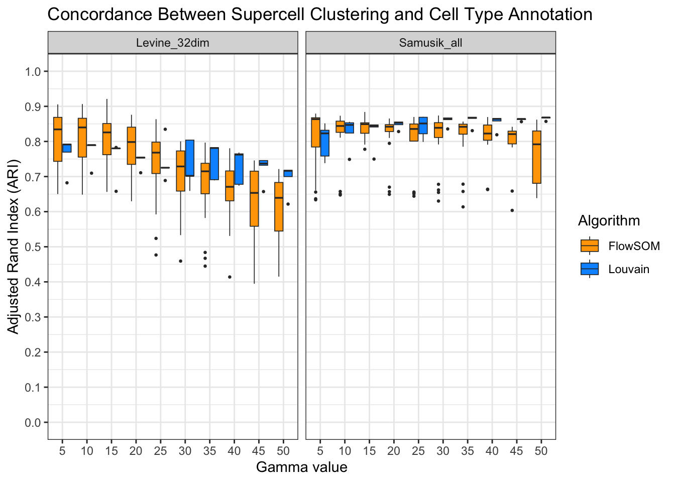
ARI between Supercell Clustering and Ground Truth Annotation

algo <- c("flowsom", "louvain")
levine_ari <- rbindlist(lapply(algo, function(alg) {
  res <- fread(here(levine_res_dir, "evaluation", paste0(alg, "_ari_vs_truth.csv")))
  res <- res[, c("gamma", "ari"), with = FALSE]
  res[, algorithm := str_to_title(alg)]
  res[, dataset := "Levine_32dim"]
  return(res)
}))
samusik_ari <- rbindlist(lapply(algo, function(alg) {
  res <- fread(here(samusik_res_dir, "evaluation", paste0(alg, "_ari_vs_truth.csv")))
  res <- res[, c("gamma", "ari"), with = FALSE]
  res[, algorithm := str_to_title(alg)]
  res[, dataset := "Samusik_all"]
}))
ari_truth <- rbind(levine_ari, samusik_ari)
ari_truth[, algorithm := ifelse(algorithm == "Flowsom", "FlowSOM", algorithm)]

ggplot(ari_truth, aes(x = factor(gamma), y = ari, fill = algorithm)) +
  geom_boxplot(outlier.size = 0.5, lwd = 0.3) +
  facet_wrap(~dataset) +
  theme_bw() +
  scale_y_continuous(breaks = pretty_breaks(n = 10), limits = c(0, 1)) +
  scale_fill_manual(values = c("FlowSOM" = "orange", "Louvain" = "#0096FF")) +
  labs(
    y = "Adjusted Rand Index (ARI)", x = "Gamma value", fill = "Algorithm",
    title = "Concordance Between Supercell Clustering and Cell Type Annotation"
  )

Version	Author	Date
366514e	Givanna Putri	2023-07-28

High scores across all datasets, clustering algorithms, and gamma values

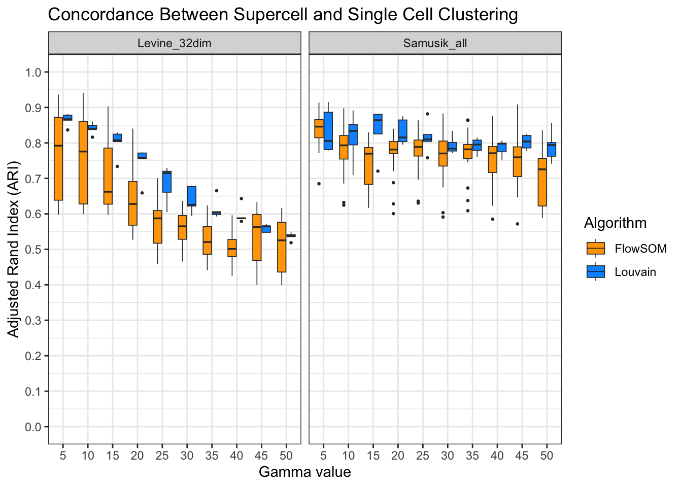
ARI between Supercell and Single Cell Clustering

algo <- c("flowsom", "louvain")
levine_ari <- rbindlist(lapply(algo, function(alg) {
  res <- fread(here(levine_res_dir, "evaluation", paste0(alg, "_ari_vs_all.csv")))
  res <- res[, c("gamma", "ari"), with = FALSE]
  res[, algorithm := str_to_title(alg)]
  res[, dataset := "Levine_32dim"]
  return(res)
}))
samusik_ari <- rbindlist(lapply(algo, function(alg) {
  res <- fread(here(samusik_res_dir, "evaluation", paste0(alg, "_ari_vs_all.csv")))
  res <- res[, c("gamma", "ari"), with = FALSE]
  res[, algorithm := str_to_title(alg)]
  res[, dataset := "Samusik_all"]
}))
ari_all <- rbind(levine_ari, samusik_ari)
ari_all[, algorithm := ifelse(algorithm == "Flowsom", "FlowSOM", algorithm)]

ggplot(ari_all, aes(x = factor(gamma), y = ari, fill = algorithm)) +
  geom_boxplot(outlier.size = 0.5, lwd = 0.3) +
  facet_wrap(~dataset) +
  theme_bw() +
  scale_y_continuous(breaks = pretty_breaks(n = 10), limits = c(0, 1)) +
  scale_fill_manual(values = c("FlowSOM" = "orange", "Louvain" = "#0096FF")) +
  labs(
    y = "Adjusted Rand Index (ARI)", x = "Gamma value", fill = "Algorithm",
    title = "Concordance Between Supercell and Single Cell Clustering"
  )

Version	Author	Date
366514e	Givanna Putri	2023-07-28

High scores across all datasets, clustering algorithms, and gamma values.

References

Levine, Jacob H, Erin F Simonds, Sean C Bendall, Kara L Davis, D Amir El-ad, Michelle D Tadmor, Oren Litvin, et al. 2015. “Data-Driven Phenotypic Dissection of AML Reveals Progenitor-Like Cells That Correlate with Prognosis.” Cell 162 (1): 184–97.

Samusik, Nikolay, Zinaida Good, Matthew H Spitzer, Kara L Davis, and Garry P Nolan. 2016. “Automated Mapping of Phenotype Space with Single-Cell Data.” Nature Methods 13 (6): 493–96.

Weber, Lukas M, and Mark D Robinson. 2016. “Comparison of Clustering Methods for High-Dimensional Single-Cell Flow and Mass Cytometry Data.” Cytometry Part A 89 (12): 1084–96.

sessionInfo()

R version 4.2.3 (2023-03-15)
Platform: aarch64-apple-darwin20 (64-bit)
Running under: macOS 14.0

Matrix products: default
BLAS:   /Library/Frameworks/R.framework/Versions/4.2-arm64/Resources/lib/libRblas.0.dylib
LAPACK: /Library/Frameworks/R.framework/Versions/4.2-arm64/Resources/lib/libRlapack.dylib

locale:
[1] en_US.UTF-8/en_US.UTF-8/en_US.UTF-8/C/en_US.UTF-8/en_US.UTF-8

attached base packages:
[1] stats     graphics  grDevices utils     datasets  methods   base     

other attached packages:
[1] viridis_0.6.2      viridisLite_0.4.1  ggridges_0.5.4     stringr_1.5.0     
[5] here_1.0.1         scales_1.2.1       ggplot2_3.4.1      data.table_1.14.10
[9] workflowr_1.7.0   

loaded via a namespace (and not attached):
 [1] tidyselect_1.2.0 xfun_0.39        bslib_0.4.2      colorspace_2.1-0
 [5] vctrs_0.5.2      generics_0.1.3   htmltools_0.5.4  yaml_2.3.7      
 [9] utf8_1.2.3       rlang_1.0.6      jquerylib_0.1.4  later_1.3.0     
[13] pillar_1.8.1     glue_1.6.2       withr_2.5.0      lifecycle_1.0.3 
[17] munsell_0.5.0    gtable_0.3.1     evaluate_0.20    knitr_1.42      
[21] callr_3.7.3      fastmap_1.1.0    httpuv_1.6.9     ps_1.7.2        
[25] fansi_1.0.4      highr_0.10       Rcpp_1.0.10      promises_1.2.0.1
[29] cachem_1.0.6     jsonlite_1.8.4   farver_2.1.1     fs_1.6.1        
[33] gridExtra_2.3    digest_0.6.31    stringi_1.7.12   processx_3.8.0  
[37] dplyr_1.1.0      getPass_0.2-2    rprojroot_2.0.3  grid_4.2.3      
[41] cli_3.6.1        tools_4.2.3      magrittr_2.0.3   sass_0.4.5      
[45] tibble_3.1.8     whisker_0.4.1    pkgconfig_2.0.3  rmarkdown_2.20  
[49] httr_1.4.4       rstudioapi_0.14  R6_2.5.1         git2r_0.31.0    
[53] compiler_4.2.3

Supercells Preserve Biological Heterogeneity and Facilitate Efficient Cell Type Identification

Givanna Putri

2023-05-23