Simulations with true cell type proportion differences

workflowr

• Summary
• Checks
• Past versions

Last updated: 2022-08-18

Checks: 7 0

Knit directory: propeller-paper-analysis/

This reproducible R Markdown analysis was created with workflowr (version 1.7.0). The Checks tab describes the reproducibility checks that were applied when the results were created. The Past versions tab lists the development history.

---

R Markdown file: up-to-date

Great! Since the R Markdown file has been committed to the Git repository, you know the exact version of the code that produced these results.

Environment: empty

Great job! The global environment was empty. Objects defined in the global environment can affect the analysis in your R Markdown file in unknown ways. For reproduciblity it’s best to always run the code in an empty environment.

Seed: set.seed(20220531)

The command set.seed(20220531) was run prior to running the code in the R Markdown file. Setting a seed ensures that any results that rely on randomness, e.g. subsampling or permutations, are reproducible.

Session information: recorded

Great job! Recording the operating system, R version, and package versions is critical for reproducibility.

Cache: none

Nice! There were no cached chunks for this analysis, so you can be confident that you successfully produced the results during this run.

File paths: relative

Great job! Using relative paths to the files within your workflowr project makes it easier to run your code on other machines.

Repository version: 2586453

Great! You are using Git for version control. Tracking code development and connecting the code version to the results is critical for reproducibility.

The results in this page were generated with repository version 2586453. See the Past versions tab to see a history of the changes made to the R Markdown and HTML files.

Note that you need to be careful to ensure that all relevant files for the analysis have been committed to Git prior to generating the results (you can use wflow_publish or wflow_git_commit). workflowr only checks the R Markdown file, but you know if there are other scripts or data files that it depends on. Below is the status of the Git repository when the results were generated:

Ignored files:
    Ignored:    .Rhistory
    Ignored:    .Rproj.user/
    Ignored:    data/cold_warm_fresh_cellinfo.txt
    Ignored:    data/covid.cell.annotation.meta.txt
    Ignored:    data/heartFYA.Rds
    Ignored:    data/pool_1.rds

Untracked files:
    Untracked:  analysis/PlotsForPaper.Rmd
    Untracked:  code/SimCode.R
    Untracked:  code/SimCodeTrueDiff.R
    Untracked:  code/auroc.R
    Untracked:  code/convertData.R
    Untracked:  data/CTpropsTransposed.txt
    Untracked:  data/CelltypeLevels.csv
    Untracked:  data/TypeIErrTables.Rdata
    Untracked:  data/appnote1cdata.rdata
    Untracked:  data/cellinfo.csv
    Untracked:  data/nullsimsVaryN_results.Rdata
    Untracked:  data/sampleinfo.csv
    Untracked:  output/1x/
    Untracked:  output/Fig1ab.pdf
    Untracked:  output/Fig1cde.pdf
    Untracked:  output/Fig2ab.pdf
    Untracked:  output/Fig2abc.pdf
    Untracked:  output/Fig2c.pdf
    Untracked:  output/Figure1.pdf
    Untracked:  output/Figure1.png
    Untracked:  output/Figure2-01.png
    Untracked:  output/Figure2-with#.pdf
    Untracked:  output/Figure2-with#.png
    Untracked:  output/Figure2.ai
    Untracked:  output/Figure2.pdf
    Untracked:  output/Figure2.png
    Untracked:  output/Figure2_E_annotatedwithProp.pdf
    Untracked:  output/Figure3.pdf
    Untracked:  output/Figure3.png
    Untracked:  output/PDF/
    Untracked:  output/SuppFig4.pdf
    Untracked:  output/SuppFig4.png
    Untracked:  output/SuppTrueDiff10.pdf
    Untracked:  output/SuppTrueDiff20.pdf
    Untracked:  output/SuppTrueDiff3.pdf
    Untracked:  output/Supplementary Figure 2 v2.png
    Untracked:  output/Supplementary Figure 2.ai
    Untracked:  output/Supplementary Figure 2.pdf
    Untracked:  output/Supplementary Figure 2.png
    Untracked:  output/SupplementaryFigure3.pdf
    Untracked:  output/TrueDiffSimResults.Rda
    Untracked:  output/covidResults.pdf
    Untracked:  output/example_simdata.pdf
    Untracked:  output/extremeCaseTrueProps20CT.pdf
    Untracked:  output/fig2d.pdf
    Untracked:  output/gude-2022-06-27.log
    Untracked:  output/gude-2022-06-29.log
    Untracked:  output/heartResults.pdf
    Untracked:  output/heatmap20CT.pdf
    Untracked:  output/legend-fig2d.pdf
    Untracked:  output/pbmcOldYoungResults.pdf
    Untracked:  output/type1error5.csv
    Untracked:  output/typeIerrorResults.Rda

Note that any generated files, e.g. HTML, png, CSS, etc., are not included in this status report because it is ok for generated content to have uncommitted changes.

---

These are the previous versions of the repository in which changes were made to the R Markdown (analysis/SimTrueDiff.Rmd) and HTML (docs/SimTrueDiff.html) files. If you’ve configured a remote Git repository (see ?wflow_git_remote), click on the hyperlinks in the table below to view the files as they were in that past version.

File	Version	Author	Date	Message
Rmd	2586453	bphipson	2022-08-18	update analysis scripts
html	67456c7	bphipson	2022-06-03	Build site.
Rmd	b239441	bphipson	2022-06-03	update simulations
html	2313cc7	bphipson	2022-06-01	Build site.
Rmd	7ec7a76	bphipson	2022-06-01	Add null simulation results and true difference simulation results

---

Load the libraries

library(speckle)
library(limma)
library(edgeR)
library(pheatmap)
library(gt)

Source the simulation code:

source("./code/SimCodeTrueDiff.R")
source("./code/auroc.R")

Hierarchical model for simulating cell type proportions

I am simulating cell type proportions in a hierarchical manner.

• The total number of cells, \(n_j\), for each sample \(j\), are drawn from a negative binomial distribution with mean 5000 and dispersion 20.
• The true cell type proportions for 7 cell types are estimated from a human heart dataset
• The sample proportion \(p_{ij}\) for cell type \(i\) and sample \(j\) is assumed to be drawn from a Beta distribution with parameters \(\alpha\) and \(\beta\).
• The count for cell type \(i\) and sample \(j\) is then drawn from a binomial distribution with probability \(p_{ij}\) and size \(n_j\).

The Beta-Binomial model allows for biological variability to be simulated between samples. The paramaters of the Beta distribution, \(\alpha\) and \(\beta\), determine how variable the \(p_{ij}\) will be. Larger values of \(\alpha\) and \(\beta\) result in a more precise distribution centred around the true proportions, while smaller values result in a more diffuse prior. The parameters for the Beta distribution were estimated from the cell type counts observed in the human heart dataset using the function estimateBetaParamsFromCounts in the speckle package.

Two group simulation set up

I will generate cell type counts for 7 cell types, assuming two experimental groups with a sample size of n=(3,5,10,20) in each group. I will calculate p-values from the following models:

• propeller (arcsin sqrt transformation)
• propeller (logit transformation)
• chi-square test of differences in proportions
• beta-binomial model using alternative parameterisation in edgeR
• logistic binomial regression (beta-binomial with dispersion=0)
• negative binomial regression (LRT and QLF in edgeR)
• Poisson regression (negative binomial with dispersion=0)
• CODA model

One thousand simulation datasets will be generated.

First I set up the simulation parameters and set up the objects to capture the output.

# Sim parameters
set.seed(10)
nsim <- 1000
depth <- 5000

# True cell type proportions from human heart dataset
heart.info <- read.csv(file="./data/cellinfo.csv", row.names = 1)
heart.counts <- table(heart.info$Celltype, heart.info$Sample)
heart.counts <- heart.counts[-4,]
trueprops <- rowSums(heart.counts)/sum(rowSums(heart.counts))

betaparams <- estimateBetaParamsFromCounts(heart.counts)

# Parameters for beta distribution
a <- betaparams$alpha
b <- betaparams$beta

# Decide on what output to keep
pval.chsq <- pval.bb <- pval.lb <- pval.nb <- pval.qlf <- pval.pois <- pval.logit <-  pval.asin <- 
  pval.coda <- matrix(NA,nrow=length(trueprops),ncol=nsim)

Set up true proportions for the two groups:

# Set up true props for the two groups
grp1.trueprops <- grp2.trueprops <- trueprops
grp2.trueprops[1] <- grp1.trueprops[1]/2
grp2.trueprops[4] <- grp2.trueprops[4]*2
grp2.trueprops[7] <- grp1.trueprops[7]*3

grp2.trueprops[1] <- grp2.trueprops[1] + (1-sum(grp2.trueprops))/2
grp2.trueprops[4] <- grp2.trueprops[4] + (1-sum(grp2.trueprops))
 
sum(grp1.trueprops)

[1] 1

sum(grp2.trueprops)

[1] 1

da.fac <- grp2.trueprops/grp1.trueprops

o <- order(trueprops)
par(mar=c(9,5,2,2))
barplot(t(cbind(grp1.trueprops[o],grp2.trueprops[o])), beside=TRUE, col=c(2,4), 
        las=2, ylab="True cell type proportion")
legend("topleft", fill=c(2,4),legend=c("Group 1","Group 2"))
title("True cell type proportions for Group 1 and 2")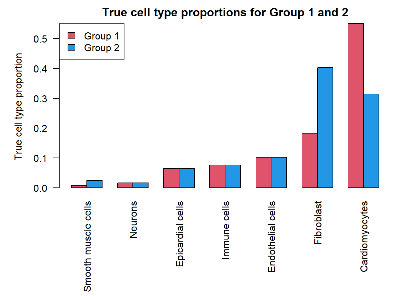

# Get hyperparameters for alpha and beta
# Note group 1 and group 2 have different b parameters to accommodate true
# differences in cell type proportions
a <- a
b.grp1 <- a*(1-grp1.trueprops)/grp1.trueprops
b.grp2 <- a*(1-grp2.trueprops)/grp2.trueprops

Next we simulate the cell type counts and run the various statistical models for testing cell type proportion differences between the two groups. We expect to see significant differences in cell type proportions in three cell types, and no significant differences in the remaining four cell types between group 1 and group 2. We expect differences in the Smooth muscle cells (most rare), Fibroblasts (second most abundant) and Cardiomyocytes (most abundant).

Sample size of 3 in each group

nsamp <- 6

for(i in 1:nsim){
    #Simulate cell type counts
    counts <- SimulateCellCountsTrueDiff(props=trueprops,nsamp=nsamp,depth=depth,a=a,
                                         b.grp1=b.grp1,b.grp2=b.grp2)

    tot.cells <- colSums(counts)
    # propeller
    est.props <- t(t(counts)/tot.cells)
    
    #asin transform
    trans.prop <- asin(sqrt(est.props))
    
    #logit transform
    nc <- normCounts(counts)
    est.props.logit <- t(t(nc+0.5)/(colSums(nc+0.5)))
    logit.prop <- log(est.props.logit/(1-est.props.logit))

    grp <- rep(c(0,1), each=nsamp/2)
    des <- model.matrix(~grp)
  
    # asinsqrt transform
    fit <- lmFit(trans.prop, des)
    fit <- eBayes(fit, robust=TRUE)

    pval.asin[,i] <- fit$p.value[,2]
    
    # logit transform
    fit.logit <- lmFit(logit.prop, des)
    fit.logit <- eBayes(fit.logit, robust=TRUE)

    pval.logit[,i] <- fit.logit$p.value[,2]

    # Chi-square test for differences in proportions
    n <- tapply(tot.cells, grp, sum)
    for(h in 1:nrow(counts)){
        pval.chsq[h,i] <- prop.test(tapply(counts[h,],grp,sum),n)$p.value
    }

    # Beta binomial implemented in edgeR (methylation workflow)
    meth.counts <- counts
    unmeth.counts <- t(tot.cells - t(counts))
    new.counts <- cbind(meth.counts,unmeth.counts)
    sam.info <- data.frame(Sample = rep(1:nsamp,2), Group=rep(grp,2), Meth = rep(c("me","un"), each=nsamp))

    design.samples <- model.matrix(~0+factor(sam.info$Sample))
    colnames(design.samples) <- paste("S",1:nsamp,sep="")
    design.group <- model.matrix(~0+factor(sam.info$Group))   
    colnames(design.group) <- c("A","B")
    design.bb <- cbind(design.samples, (sam.info$Meth=="me") * design.group)
    lib.size = rep(tot.cells,2)

    y <- DGEList(new.counts)
    y$samples$lib.size <- lib.size
    y <- estimateDisp(y, design.bb, trend="none")
    fit.bb <- glmFit(y, design.bb)
    contr <- makeContrasts(Grp=B-A, levels=design.bb)
    lrt <- glmLRT(fit.bb, contrast=contr)
    pval.bb[,i] <- lrt$table$PValue

    # Logistic binomial regression
    fit.lb <- glmFit(y, design.bb, dispersion = 0)
    lrt.lb <- glmLRT(fit.lb, contrast=contr)
    pval.lb[,i] <- lrt.lb$table$PValue

    # Negative binomial
    y.nb <- DGEList(counts)
    y.nb <- estimateDisp(y.nb, des, trend="none")
    fit.nb <- glmFit(y.nb, des)
    lrt.nb <- glmLRT(fit.nb, coef=2)
    pval.nb[,i] <- lrt.nb$table$PValue
    
    # Negative binomial QLF test
    fit.qlf <- glmQLFit(y.nb, des, robust=TRUE, abundance.trend = FALSE)
    res.qlf <- glmQLFTest(fit.qlf, coef=2)
    pval.qlf[,i] <- res.qlf$table$PValue

    # Poisson
    fit.poi <- glmFit(y.nb, des, dispersion = 0)
    lrt.poi <- glmLRT(fit.poi, coef=2)
    pval.pois[,i] <- lrt.poi$table$PValue
    
    # CODA
    # Replace zero counts with 0.5 so that the geometric mean always works
    if(any(counts==0)) counts[counts==0] <- 0.5
    geomean <- apply(counts,2, function(x) exp(mean(log(x))))
    geomean.mat <- expandAsMatrix(geomean,dim=c(nrow(counts),ncol(counts)),byrow = FALSE)
    clr <- counts/geomean.mat
    logratio <- log(clr)
    
    fit.coda <- lmFit(logratio, des)
    fit.coda <- eBayes(fit.coda, robust=TRUE)

    pval.coda[,i] <- fit.coda$p.value[,2]

}

We can look at the number of significant tests at certain p-value cut-offs:

pcut <- 0.05
de <- da.fac != 1
sig.disc <- matrix(NA,nrow=length(trueprops),ncol=9)
rownames(sig.disc) <- names(trueprops)
colnames(sig.disc) <- c("chisq","logbin","pois","asin", "logit","betabin","negbin","nbQLF","CODA")

sig.disc[,1]<-rowSums(pval.chsq<pcut)/nsim 
sig.disc[,2]<-rowSums(pval.lb<pcut)/nsim
sig.disc[,3]<-rowSums(pval.pois<pcut)/nsim 
sig.disc[,4]<-rowSums(pval.asin<pcut)/nsim 
sig.disc[,5]<-rowSums(pval.logit<pcut)/nsim 
sig.disc[,6]<-rowSums(pval.bb<pcut)/nsim
sig.disc[,7]<-rowSums(pval.nb<pcut)/nsim 
sig.disc[,8]<-rowSums(pval.qlf<pcut)/nsim
sig.disc[,9]<-rowSums(pval.coda<pcut)/nsim 
o <- order(trueprops)

gt(data.frame(sig.disc[o,]),rownames_to_stub = TRUE, caption="Proportion of significant tests: n=3")

Proportion of significant tests: n=3

	chisq	logbin	pois	asin	logit	betabin	negbin	nbQLF	CODA
Smooth muscle cells	0.964	0.967	0.966	0.210	0.530	0.570	0.643	0.580	0.491
Neurons	0.736	0.741	0.740	0.020	0.079	0.097	0.119	0.097	0.097
Epicardial cells	0.868	0.869	0.866	0.042	0.037	0.046	0.064	0.049	0.059
Immune cells	0.908	0.908	0.905	0.102	0.119	0.137	0.139	0.116	0.124
Endothelial cells	0.805	0.806	0.798	0.042	0.016	0.017	0.018	0.018	0.023
Fibroblast	0.998	0.998	0.997	0.643	0.539	0.594	0.442	0.407	0.275
Cardiomyocytes	0.996	0.996	0.995	0.581	0.479	0.532	0.247	0.223	0.405

layout(matrix(c(1,1,1,2), 1, 4, byrow = TRUE))
par(mar=c(8,5,3,2))
par(mgp=c(3, 0.5, 0))
o <- order(trueprops)
names <- c("propeller (asin)","propeller (logit)","betabin","negbin","negbinQLF","CODA")
barplot(sig.disc[o,4:9],beside=TRUE,col=ggplotColors(length(b)),
        ylab="Proportion sig. tests", names=names,
        cex.axis = 1.5, cex.lab=1.5, cex.names = 1.35, ylim=c(0,1), las=2)
title(paste("Significant tests, n=",nsamp/2,sep=""), cex.main=1.5)
abline(h=pcut,lty=2,lwd=2)
par(mar=c(0,0,0,0))
plot(1, type = "n", xlab = "", ylab = "", xaxt="n",yaxt="n", bty="n")
legend("center", legend=paste("True p =",round(trueprops,3)[o]), fill=ggplotColors(length(b)), cex=1.5)

o <- order(trueprops)
mysig <- sig.disc[o,4:9]
colnames(mysig) <- names
pheatmap(mysig, scale="none", cluster_rows = FALSE, cluster_cols = FALSE,
         labels_row = c(expression(paste(pi, " = 0.008*", sep="")),
                        expression(paste(pi, " = 0.016", sep="")),
                        expression(paste(pi, " = 0.064", sep="")),
                        expression(paste(pi, " = 0.076", sep="")),
                        expression(paste(pi, " = 0.102", sep="")),
                        expression(paste(pi, " = 0.183*", sep="")),
                        expression(paste(pi, " = 0.551*", sep=""))),
         main=paste("Significant tests, n=",nsamp/2,sep=""))

auc.asin <- auc.logit <- auc.bb <- auc.nb <- auc.qlf <- auc.coda <- rep(NA,nsim)
for(i in 1:nsim){
  auc.asin[i] <- auroc(score=1-pval.asin[,i],bool=de)
  auc.logit[i] <- auroc(score=1-pval.logit[,i],bool=de)
  auc.bb[i] <- auroc(score=1-pval.bb[,i],bool=de)
  auc.nb[i] <- auroc(score=1-pval.nb[,i],bool=de)
  auc.qlf[i] <- auroc(score=1-pval.qlf[,i],bool=de)
  auc.coda[i] <- auroc(score=1-pval.coda[,i],bool=de)
}

mean(auc.asin)

[1] 0.8560833

mean(auc.logit)

[1] 0.85875

mean(auc.bb)

[1] 0.8645833

mean(auc.nb)

[1] 0.823

mean(auc.qlf)

[1] 0.8266667

mean(auc.coda)

[1] 0.7779167

auc.mat <- matrix(NA,ncol=6,nrow=4)
rownames(auc.mat) <- c("n=3","n=5","n=10","n=20")
colnames(auc.mat) <- names
auc.mat[1,1] <- mean(auc.asin)
auc.mat[1,2] <- mean(auc.logit)
auc.mat[1,3] <- mean(auc.bb)
auc.mat[1,4] <- mean(auc.nb)
auc.mat[1,5] <- mean(auc.qlf)
auc.mat[1,6] <- mean(auc.coda)

par(mfrow=c(1,1))
par(mar=c(9,5,3,2))
barplot(c(mean(auc.asin),mean(auc.logit),mean(auc.bb),mean(auc.nb),mean(auc.qlf),mean(auc.coda)), ylim=c(0,1), ylab= "AUC", cex.axis=1.5, cex.lab=1.5, names=names, las=2, cex.names = 1.5)
title(paste("AUC: sample size n=",nsamp/2,sep=""),cex.main=1.5)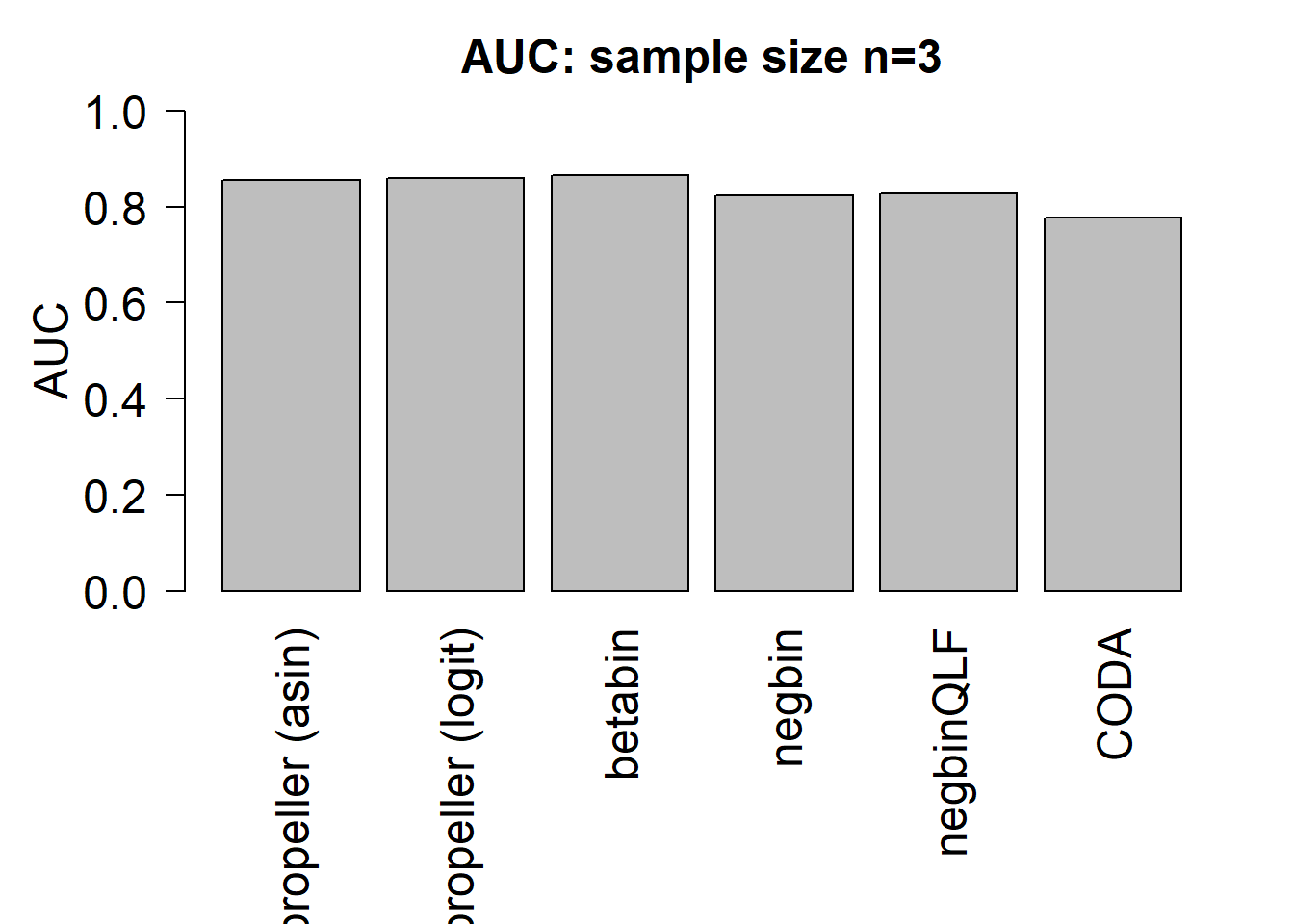

sig.disc3 <- sig.disc

Sample size of 5 in each group

nsamp <- 10

for(i in 1:nsim){
    #Simulate cell type counts
    counts <- SimulateCellCountsTrueDiff(props=trueprops,nsamp=nsamp,depth=depth,a=a,
                                         b.grp1=b.grp1,b.grp2=b.grp2)

    tot.cells <- colSums(counts)
    # propeller
    est.props <- t(t(counts)/tot.cells)
    
    #asin transform
    trans.prop <- asin(sqrt(est.props))
    
    #logit transform
    nc <- normCounts(counts)
    est.props.logit <- t(t(nc+0.5)/(colSums(nc+0.5)))
    logit.prop <- log(est.props.logit/(1-est.props.logit))

    grp <- rep(c(0,1), each=nsamp/2)
    des <- model.matrix(~grp)
  
    # asinsqrt transform
    fit <- lmFit(trans.prop, des)
    fit <- eBayes(fit, robust=TRUE)

    pval.asin[,i] <- fit$p.value[,2]
    
    # logit transform
    fit.logit <- lmFit(logit.prop, des)
    fit.logit <- eBayes(fit.logit, robust=TRUE)

    pval.logit[,i] <- fit.logit$p.value[,2]

    # Chi-square test for differences in proportions
    n <- tapply(tot.cells, grp, sum)
    for(h in 1:nrow(counts)){
        pval.chsq[h,i] <- prop.test(tapply(counts[h,],grp,sum),n)$p.value
    }

    # Beta binomial implemented in edgeR (methylation workflow)
    meth.counts <- counts
    unmeth.counts <- t(tot.cells - t(counts))
    new.counts <- cbind(meth.counts,unmeth.counts)
    sam.info <- data.frame(Sample = rep(1:nsamp,2), Group=rep(grp,2), Meth = rep(c("me","un"), each=nsamp))

    design.samples <- model.matrix(~0+factor(sam.info$Sample))
    colnames(design.samples) <- paste("S",1:nsamp,sep="")
    design.group <- model.matrix(~0+factor(sam.info$Group))   
    colnames(design.group) <- c("A","B")
    design.bb <- cbind(design.samples, (sam.info$Meth=="me") * design.group)
    lib.size = rep(tot.cells,2)

    y <- DGEList(new.counts)
    y$samples$lib.size <- lib.size
    y <- estimateDisp(y, design.bb, trend="none")
    fit.bb <- glmFit(y, design.bb)
    contr <- makeContrasts(Grp=B-A, levels=design.bb)
    lrt <- glmLRT(fit.bb, contrast=contr)
    pval.bb[,i] <- lrt$table$PValue

    # Logistic binomial regression
    fit.lb <- glmFit(y, design.bb, dispersion = 0)
    lrt.lb <- glmLRT(fit.lb, contrast=contr)
    pval.lb[,i] <- lrt.lb$table$PValue

    # Negative binomial
    y.nb <- DGEList(counts)
    y.nb <- estimateDisp(y.nb, des, trend="none")
    fit.nb <- glmFit(y.nb, des)
    lrt.nb <- glmLRT(fit.nb, coef=2)
    pval.nb[,i] <- lrt.nb$table$PValue
    
    # Negative binomial QLF test
    fit.qlf <- glmQLFit(y.nb, des, robust=TRUE, abundance.trend = FALSE)
    res.qlf <- glmQLFTest(fit.qlf, coef=2)
    pval.qlf[,i] <- res.qlf$table$PValue

    # Poisson
    fit.poi <- glmFit(y.nb, des, dispersion = 0)
    lrt.poi <- glmLRT(fit.poi, coef=2)
    pval.pois[,i] <- lrt.poi$table$PValue
    
    # CODA
    # Replace zero counts with 0.5 so that the geometric mean always works
    if(any(counts==0)) counts[counts==0] <- 0.5
    geomean <- apply(counts,2, function(x) exp(mean(log(x))))
    geomean.mat <- expandAsMatrix(geomean,dim=c(nrow(counts),ncol(counts)),byrow = FALSE)
    clr <- counts/geomean.mat
    logratio <- log(clr)
    
    fit.coda <- lmFit(logratio, des)
    fit.coda <- eBayes(fit.coda, robust=TRUE)

    pval.coda[,i] <- fit.coda$p.value[,2]

}

We can look at the number of significant tests at certain p-value cut-offs:

pcut <- 0.05
de <- da.fac != 1
sig.disc <- matrix(NA,nrow=length(trueprops),ncol=9)
rownames(sig.disc) <- names(trueprops)
colnames(sig.disc) <- c("chisq","logbin","pois","asin", "logit","betabin","negbin","nbQLF","CODA")

sig.disc[,1]<-rowSums(pval.chsq<pcut)/nsim 
sig.disc[,2]<-rowSums(pval.lb<pcut)/nsim
sig.disc[,3]<-rowSums(pval.pois<pcut)/nsim 
sig.disc[,4]<-rowSums(pval.asin<pcut)/nsim 
sig.disc[,5]<-rowSums(pval.logit<pcut)/nsim 
sig.disc[,6]<-rowSums(pval.bb<pcut)/nsim
sig.disc[,7]<-rowSums(pval.nb<pcut)/nsim 
sig.disc[,8]<-rowSums(pval.qlf<pcut)/nsim
sig.disc[,9]<-rowSums(pval.coda<pcut)/nsim 
o <- order(trueprops)

gt(data.frame(sig.disc[o,]),rownames_to_stub = TRUE, caption="Proportion of significant tests: n=5")

Proportion of significant tests: n=5

	chisq	logbin	pois	asin	logit	betabin	negbin	nbQLF	CODA
Smooth muscle cells	0.994	0.994	0.994	0.522	0.737	0.762	0.813	0.771	0.715
Neurons	0.742	0.745	0.744	0.024	0.071	0.081	0.105	0.090	0.095
Epicardial cells	0.847	0.849	0.840	0.053	0.050	0.055	0.069	0.058	0.081
Immune cells	0.903	0.903	0.901	0.083	0.112	0.126	0.113	0.094	0.128
Endothelial cells	0.824	0.824	0.813	0.048	0.013	0.016	0.027	0.024	0.053
Fibroblast	0.998	0.998	0.998	0.816	0.775	0.812	0.724	0.689	0.474
Cardiomyocytes	0.998	0.998	0.998	0.737	0.707	0.729	0.484	0.469	0.626

layout(matrix(c(1,1,1,2), 1, 4, byrow = TRUE))
par(mar=c(8,5,3,2))
par(mgp=c(3, 0.5, 0))
o <- order(trueprops)
names <- c("propeller (asin)","propeller (logit)","betabin","negbin","negbinQLF","CODA")
barplot(sig.disc[o,4:9],beside=TRUE,col=ggplotColors(length(b)),
        ylab="Proportion sig. tests", names=names,
        cex.axis = 1.5, cex.lab=1.5, cex.names = 1.35, ylim=c(0,1), las=2)
title(paste("Significant tests, n=",nsamp/2,sep=""), cex.main=1.5)
abline(h=pcut,lty=2,lwd=2)
par(mar=c(0,0,0,0))
plot(1, type = "n", xlab = "", ylab = "", xaxt="n",yaxt="n", bty="n")
legend("center", legend=paste("True p =",round(trueprops,3)[o]), fill=ggplotColors(length(b)), cex=1.5)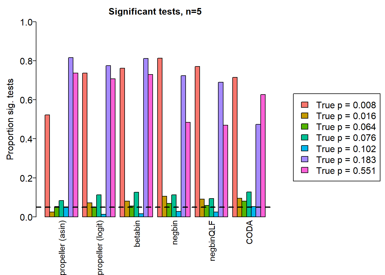

o <- order(trueprops)
mysig <- sig.disc[o,4:9]
colnames(mysig) <- names
pheatmap(mysig, scale="none", cluster_rows = FALSE, cluster_cols = FALSE,
         labels_row = c(expression(paste(pi, " = 0.008*", sep="")),
                        expression(paste(pi, " = 0.016", sep="")),
                        expression(paste(pi, " = 0.064", sep="")),
                        expression(paste(pi, " = 0.076", sep="")),
                        expression(paste(pi, " = 0.102", sep="")),
                        expression(paste(pi, " = 0.183*", sep="")),
                        expression(paste(pi, " = 0.551*", sep=""))),
         main=paste("Significant tests, n=",nsamp/2,sep=""))

auc.asin <- auc.logit <- auc.bb <- auc.nb <- auc.qlf <- auc.coda <- rep(NA,nsim)
for(i in 1:nsim){
  auc.asin[i] <- auroc(score=1-pval.asin[,i],bool=de)
  auc.logit[i] <- auroc(score=1-pval.logit[,i],bool=de)
  auc.bb[i] <- auroc(score=1-pval.bb[,i],bool=de)
  auc.nb[i] <- auroc(score=1-pval.nb[,i],bool=de)
  auc.qlf[i] <- auroc(score=1-pval.qlf[,i],bool=de)
  auc.coda[i] <- auroc(score=1-pval.coda[,i],bool=de)
}

mean(auc.asin)

[1] 0.9325833

mean(auc.logit)

[1] 0.9353333

mean(auc.bb)

[1] 0.9365833

mean(auc.nb)

[1] 0.9129167

mean(auc.qlf)

[1] 0.91525

mean(auc.coda)

[1] 0.8665833

auc.mat[2,1] <- mean(auc.asin)
auc.mat[2,2] <- mean(auc.logit)
auc.mat[2,3] <- mean(auc.bb)
auc.mat[2,4] <- mean(auc.nb)
auc.mat[2,5] <- mean(auc.qlf)
auc.mat[2,6] <- mean(auc.coda)

par(mfrow=c(1,1))
par(mar=c(9,5,3,2))
barplot(c(mean(auc.asin),mean(auc.logit),mean(auc.bb),mean(auc.nb),mean(auc.qlf),mean(auc.coda)), ylim=c(0,1), ylab= "AUC", cex.axis=1.5, cex.lab=1.5, names=names, las=2, cex.names = 1.5)
title(paste("AUC: sample size n=",nsamp/2,sep=""),cex.main=1.5)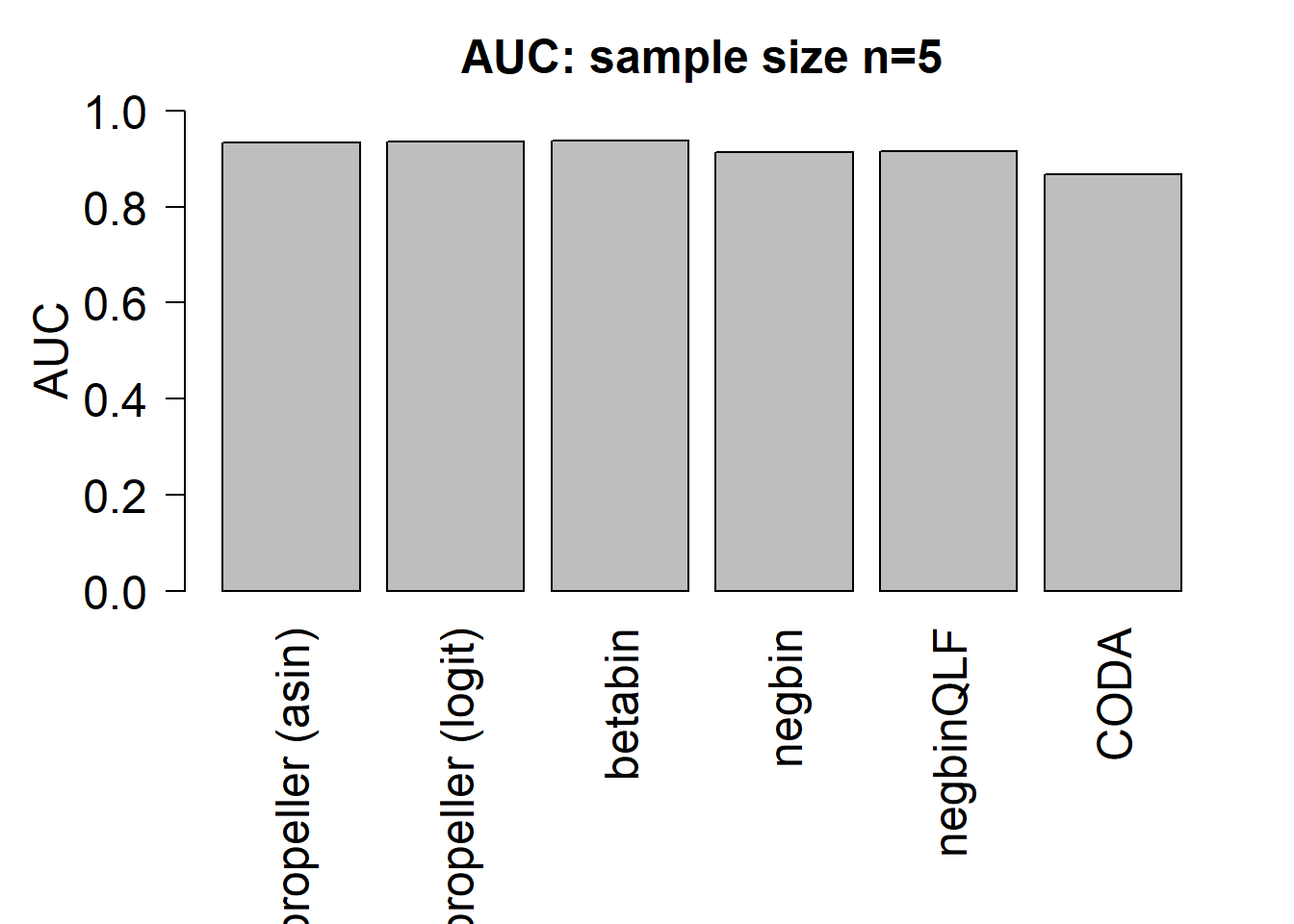

sig.disc5 <- sig.disc

Sample size of 10 in each group

nsamp <- 20

for(i in 1:nsim){
    #Simulate cell type counts
    counts <- SimulateCellCountsTrueDiff(props=trueprops,nsamp=nsamp,depth=depth,a=a,
                                         b.grp1=b.grp1,b.grp2=b.grp2)

    tot.cells <- colSums(counts)
    # propeller
    est.props <- t(t(counts)/tot.cells)
    
    #asin transform
    trans.prop <- asin(sqrt(est.props))
    
    #logit transform
    nc <- normCounts(counts)
    est.props.logit <- t(t(nc+0.5)/(colSums(nc+0.5)))
    logit.prop <- log(est.props.logit/(1-est.props.logit))

    grp <- rep(c(0,1), each=nsamp/2)
    des <- model.matrix(~grp)
  
    # asinsqrt transform
    fit <- lmFit(trans.prop, des)
    fit <- eBayes(fit, robust=TRUE)

    pval.asin[,i] <- fit$p.value[,2]
    
    # logit transform
    fit.logit <- lmFit(logit.prop, des)
    fit.logit <- eBayes(fit.logit, robust=TRUE)

    pval.logit[,i] <- fit.logit$p.value[,2]

    # Chi-square test for differences in proportions
    n <- tapply(tot.cells, grp, sum)
    for(h in 1:nrow(counts)){
        pval.chsq[h,i] <- prop.test(tapply(counts[h,],grp,sum),n)$p.value
    }

    # Beta binomial implemented in edgeR (methylation workflow)
    meth.counts <- counts
    unmeth.counts <- t(tot.cells - t(counts))
    new.counts <- cbind(meth.counts,unmeth.counts)
    sam.info <- data.frame(Sample = rep(1:nsamp,2), Group=rep(grp,2), Meth = rep(c("me","un"), each=nsamp))

    design.samples <- model.matrix(~0+factor(sam.info$Sample))
    colnames(design.samples) <- paste("S",1:nsamp,sep="")
    design.group <- model.matrix(~0+factor(sam.info$Group))   
    colnames(design.group) <- c("A","B")
    design.bb <- cbind(design.samples, (sam.info$Meth=="me") * design.group)
    lib.size = rep(tot.cells,2)

    y <- DGEList(new.counts)
    y$samples$lib.size <- lib.size
    y <- estimateDisp(y, design.bb, trend="none")
    fit.bb <- glmFit(y, design.bb)
    contr <- makeContrasts(Grp=B-A, levels=design.bb)
    lrt <- glmLRT(fit.bb, contrast=contr)
    pval.bb[,i] <- lrt$table$PValue

    # Logistic binomial regression
    fit.lb <- glmFit(y, design.bb, dispersion = 0)
    lrt.lb <- glmLRT(fit.lb, contrast=contr)
    pval.lb[,i] <- lrt.lb$table$PValue

    # Negative binomial
    y.nb <- DGEList(counts)
    y.nb <- estimateDisp(y.nb, des, trend="none")
    fit.nb <- glmFit(y.nb, des)
    lrt.nb <- glmLRT(fit.nb, coef=2)
    pval.nb[,i] <- lrt.nb$table$PValue
    
    # Negative binomial QLF test
    fit.qlf <- glmQLFit(y.nb, des, robust=TRUE, abundance.trend = FALSE)
    res.qlf <- glmQLFTest(fit.qlf, coef=2)
    pval.qlf[,i] <- res.qlf$table$PValue

    # Poisson
    fit.poi <- glmFit(y.nb, des, dispersion = 0)
    lrt.poi <- glmLRT(fit.poi, coef=2)
    pval.pois[,i] <- lrt.poi$table$PValue
    
    # CODA
    # Replace zero counts with 0.5 so that the geometric mean always works
    if(any(counts==0)) counts[counts==0] <- 0.5
    geomean <- apply(counts,2, function(x) exp(mean(log(x))))
    geomean.mat <- expandAsMatrix(geomean,dim=c(nrow(counts),ncol(counts)),byrow = FALSE)
    clr <- counts/geomean.mat
    logratio <- log(clr)
    
    fit.coda <- lmFit(logratio, des)
    fit.coda <- eBayes(fit.coda, robust=TRUE)

    pval.coda[,i] <- fit.coda$p.value[,2]

}

We can look at the number of significant tests at certain p-value cut-offs:

pcut <- 0.05
de <- da.fac != 1
sig.disc <- matrix(NA,nrow=length(trueprops),ncol=9)
rownames(sig.disc) <- names(trueprops)
colnames(sig.disc) <- c("chisq","logbin","pois","asin", "logit","betabin","negbin","nbQLF","CODA")

sig.disc[,1]<-rowSums(pval.chsq<pcut)/nsim 
sig.disc[,2]<-rowSums(pval.lb<pcut)/nsim
sig.disc[,3]<-rowSums(pval.pois<pcut)/nsim 
sig.disc[,4]<-rowSums(pval.asin<pcut)/nsim 
sig.disc[,5]<-rowSums(pval.logit<pcut)/nsim 
sig.disc[,6]<-rowSums(pval.bb<pcut)/nsim
sig.disc[,7]<-rowSums(pval.nb<pcut)/nsim 
sig.disc[,8]<-rowSums(pval.qlf<pcut)/nsim
sig.disc[,9]<-rowSums(pval.coda<pcut)/nsim 
o <- order(trueprops)

gt(data.frame(sig.disc[o,]),rownames_to_stub = TRUE, caption="Proportion of significant tests: n=10")

Proportion of significant tests: n=10

	chisq	logbin	pois	asin	logit	betabin	negbin	nbQLF	CODA
Smooth muscle cells	1.000	1.000	1.000	0.944	0.971	0.976	0.976	0.971	0.964
Neurons	0.754	0.755	0.754	0.040	0.060	0.067	0.088	0.068	0.109
Epicardial cells	0.843	0.845	0.841	0.049	0.046	0.048	0.058	0.051	0.133
Immune cells	0.889	0.889	0.887	0.061	0.073	0.083	0.075	0.059	0.115
Endothelial cells	0.796	0.796	0.787	0.040	0.015	0.015	0.022	0.022	0.143
Fibroblast	1.000	1.000	1.000	0.980	0.974	0.981	0.964	0.960	0.754
Cardiomyocytes	1.000	1.000	0.999	0.936	0.924	0.938	0.866	0.856	0.880

layout(matrix(c(1,1,1,2), 1, 4, byrow = TRUE))
par(mar=c(8,5,3,2))
par(mgp=c(3, 0.5, 0))
o <- order(trueprops)
names <- c("propeller (asin)","propeller (logit)","betabin","negbin","negbinQLF","CODA")
barplot(sig.disc[o,4:9],beside=TRUE,col=ggplotColors(length(b)),
        ylab="Proportion sig. tests", names=names,
        cex.axis = 1.5, cex.lab=1.5, cex.names = 1.35, ylim=c(0,1), las=2)
title(paste("Significant tests, n=",nsamp/2,sep=""), cex.main=1.5)
abline(h=pcut,lty=2,lwd=2)
par(mar=c(0,0,0,0))
plot(1, type = "n", xlab = "", ylab = "", xaxt="n",yaxt="n", bty="n")
legend("center", legend=paste("True p =",round(trueprops,3)[o]), fill=ggplotColors(length(b)), cex=1.5)

o <- order(trueprops)
mysig <- sig.disc[o,4:9]
colnames(mysig) <- names
pheatmap(mysig, scale="none", cluster_rows = FALSE, cluster_cols = FALSE,
         labels_row = c(expression(paste(pi, " = 0.008*", sep="")),
                        expression(paste(pi, " = 0.016", sep="")),
                        expression(paste(pi, " = 0.064", sep="")),
                        expression(paste(pi, " = 0.076", sep="")),
                        expression(paste(pi, " = 0.102", sep="")),
                        expression(paste(pi, " = 0.183*", sep="")),
                        expression(paste(pi, " = 0.551*", sep=""))),
         main=paste("Significant tests, n=",nsamp/2,sep=""))

auc.asin <- auc.logit <- auc.bb <- auc.nb <- auc.qlf <- auc.coda <- rep(NA,nsim)
for(i in 1:nsim){
  auc.asin[i] <- auroc(score=1-pval.asin[,i],bool=de)
  auc.logit[i] <- auroc(score=1-pval.logit[,i],bool=de)
  auc.bb[i] <- auroc(score=1-pval.bb[,i],bool=de)
  auc.nb[i] <- auroc(score=1-pval.nb[,i],bool=de)
  auc.qlf[i] <- auroc(score=1-pval.qlf[,i],bool=de)
  auc.coda[i] <- auroc(score=1-pval.coda[,i],bool=de)
}

mean(auc.asin)

[1] 0.9900833

mean(auc.logit)

[1] 0.9899167

mean(auc.bb)

[1] 0.99025

mean(auc.nb)

[1] 0.9848333

mean(auc.qlf)

[1] 0.98525

mean(auc.coda)

[1] 0.9490833

auc.mat[3,1] <- mean(auc.asin)
auc.mat[3,2] <- mean(auc.logit)
auc.mat[3,3] <- mean(auc.bb)
auc.mat[3,4] <- mean(auc.nb)
auc.mat[3,5] <- mean(auc.qlf)
auc.mat[3,6] <- mean(auc.coda)

par(mfrow=c(1,1))
par(mar=c(9,5,3,2))
barplot(c(mean(auc.asin),mean(auc.logit),mean(auc.bb),mean(auc.nb),mean(auc.qlf),mean(auc.coda)), ylim=c(0,1), ylab= "AUC", cex.axis=1.5, cex.lab=1.5, names=names, las=2, cex.names = 1.5)
title(paste("AUC: sample size n=",nsamp/2,sep=""),cex.main=1.5)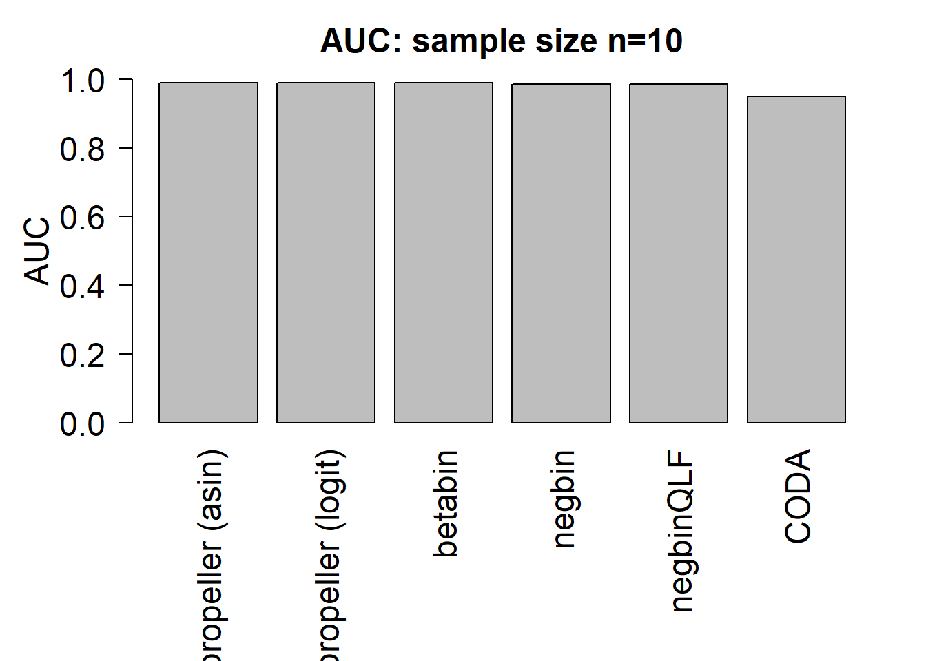

sig.disc10 <- sig.disc

Sample size of 20 in each group

nsamp <- 40

for(i in 1:nsim){
    #Simulate cell type counts
    counts <- SimulateCellCountsTrueDiff(props=trueprops,nsamp=nsamp,depth=depth,a=a,
                                         b.grp1=b.grp1,b.grp2=b.grp2)

    tot.cells <- colSums(counts)
    # propeller
    est.props <- t(t(counts)/tot.cells)
    
    #asin transform
    trans.prop <- asin(sqrt(est.props))
    
    #logit transform
    nc <- normCounts(counts)
    est.props.logit <- t(t(nc+0.5)/(colSums(nc+0.5)))
    logit.prop <- log(est.props.logit/(1-est.props.logit))

    grp <- rep(c(0,1), each=nsamp/2)
    des <- model.matrix(~grp)
  
    # asinsqrt transform
    fit <- lmFit(trans.prop, des)
    fit <- eBayes(fit, robust=TRUE)

    pval.asin[,i] <- fit$p.value[,2]
    
    # logit transform
    fit.logit <- lmFit(logit.prop, des)
    fit.logit <- eBayes(fit.logit, robust=TRUE)

    pval.logit[,i] <- fit.logit$p.value[,2]

    # Chi-square test for differences in proportions
    n <- tapply(tot.cells, grp, sum)
    for(h in 1:nrow(counts)){
        pval.chsq[h,i] <- prop.test(tapply(counts[h,],grp,sum),n)$p.value
    }

    # Beta binomial implemented in edgeR (methylation workflow)
    meth.counts <- counts
    unmeth.counts <- t(tot.cells - t(counts))
    new.counts <- cbind(meth.counts,unmeth.counts)
    sam.info <- data.frame(Sample = rep(1:nsamp,2), Group=rep(grp,2), Meth = rep(c("me","un"), each=nsamp))

    design.samples <- model.matrix(~0+factor(sam.info$Sample))
    colnames(design.samples) <- paste("S",1:nsamp,sep="")
    design.group <- model.matrix(~0+factor(sam.info$Group))   
    colnames(design.group) <- c("A","B")
    design.bb <- cbind(design.samples, (sam.info$Meth=="me") * design.group)
    lib.size = rep(tot.cells,2)

    y <- DGEList(new.counts)
    y$samples$lib.size <- lib.size
    y <- estimateDisp(y, design.bb, trend="none")
    fit.bb <- glmFit(y, design.bb)
    contr <- makeContrasts(Grp=B-A, levels=design.bb)
    lrt <- glmLRT(fit.bb, contrast=contr)
    pval.bb[,i] <- lrt$table$PValue

    # Logistic binomial regression
    fit.lb <- glmFit(y, design.bb, dispersion = 0)
    lrt.lb <- glmLRT(fit.lb, contrast=contr)
    pval.lb[,i] <- lrt.lb$table$PValue

    # Negative binomial
    y.nb <- DGEList(counts)
    y.nb <- estimateDisp(y.nb, des, trend="none")
    fit.nb <- glmFit(y.nb, des)
    lrt.nb <- glmLRT(fit.nb, coef=2)
    pval.nb[,i] <- lrt.nb$table$PValue
    
    # Negative binomial QLF test
    fit.qlf <- glmQLFit(y.nb, des, robust=TRUE, abundance.trend = FALSE)
    res.qlf <- glmQLFTest(fit.qlf, coef=2)
    pval.qlf[,i] <- res.qlf$table$PValue

    # Poisson
    fit.poi <- glmFit(y.nb, des, dispersion = 0)
    lrt.poi <- glmLRT(fit.poi, coef=2)
    pval.pois[,i] <- lrt.poi$table$PValue
    
    # CODA
    # Replace zero counts with 0.5 so that the geometric mean always works
    if(any(counts==0)) counts[counts==0] <- 0.5
    geomean <- apply(counts,2, function(x) exp(mean(log(x))))
    geomean.mat <- expandAsMatrix(geomean,dim=c(nrow(counts),ncol(counts)),byrow = FALSE)
    clr <- counts/geomean.mat
    logratio <- log(clr)
    
    fit.coda <- lmFit(logratio, des)
    fit.coda <- eBayes(fit.coda, robust=TRUE)

    pval.coda[,i] <- fit.coda$p.value[,2]

}

We can look at the number of significant tests at certain p-value cut-offs:

pcut <- 0.05
de <- da.fac != 1
sig.disc <- matrix(NA,nrow=length(trueprops),ncol=9)
rownames(sig.disc) <- names(trueprops)
colnames(sig.disc) <- c("chisq","logbin","pois","asin", "logit","betabin","negbin","nbQLF","CODA")

sig.disc[,1]<-rowSums(pval.chsq<pcut)/nsim 
sig.disc[,2]<-rowSums(pval.lb<pcut)/nsim
sig.disc[,3]<-rowSums(pval.pois<pcut)/nsim 
sig.disc[,4]<-rowSums(pval.asin<pcut)/nsim 
sig.disc[,5]<-rowSums(pval.logit<pcut)/nsim 
sig.disc[,6]<-rowSums(pval.bb<pcut)/nsim
sig.disc[,7]<-rowSums(pval.nb<pcut)/nsim 
sig.disc[,8]<-rowSums(pval.qlf<pcut)/nsim
sig.disc[,9]<-rowSums(pval.coda<pcut)/nsim 
o <- order(trueprops)

gt(data.frame(sig.disc[o,]),rownames_to_stub = TRUE, caption="Proportion of significant tests: n=20")

Proportion of significant tests: n=20

	chisq	logbin	pois	asin	logit	betabin	negbin	nbQLF	CODA
Smooth muscle cells	1.000	1.000	1.000	1.000	1.000	1.000	1.000	1.000	1.000
Neurons	0.758	0.761	0.758	0.042	0.054	0.058	0.066	0.058	0.155
Epicardial cells	0.856	0.856	0.850	0.053	0.049	0.054	0.067	0.059	0.188
Immune cells	0.915	0.916	0.910	0.056	0.063	0.066	0.058	0.038	0.116
Endothelial cells	0.826	0.826	0.814	0.057	0.028	0.027	0.049	0.047	0.341
Fibroblast	1.000	1.000	1.000	1.000	1.000	1.000	1.000	1.000	0.968
Cardiomyocytes	1.000	1.000	1.000	1.000	0.998	1.000	0.996	0.994	0.994

layout(matrix(c(1,1,1,2), 1, 4, byrow = TRUE))
par(mar=c(8,5,3,2))
par(mgp=c(3, 0.5, 0))
o <- order(trueprops)
names <- c("propeller (asin)","propeller (logit)","betabin","negbin","negbinQLF","CODA")
barplot(sig.disc[o,4:9],beside=TRUE,col=ggplotColors(length(b)),
        ylab="Proportion sig. tests", names=names,
        cex.axis = 1.5, cex.lab=1.5, cex.names = 1.35, ylim=c(0,1), las=2)
title(paste("Significant tests, n=",nsamp/2,sep=""), cex.main=1.5)
abline(h=pcut,lty=2,lwd=2)
par(mar=c(0,0,0,0))
plot(1, type = "n", xlab = "", ylab = "", xaxt="n",yaxt="n", bty="n")
legend("center", legend=paste("True p =",round(trueprops,3)[o]), fill=ggplotColors(length(b)), cex=1.5)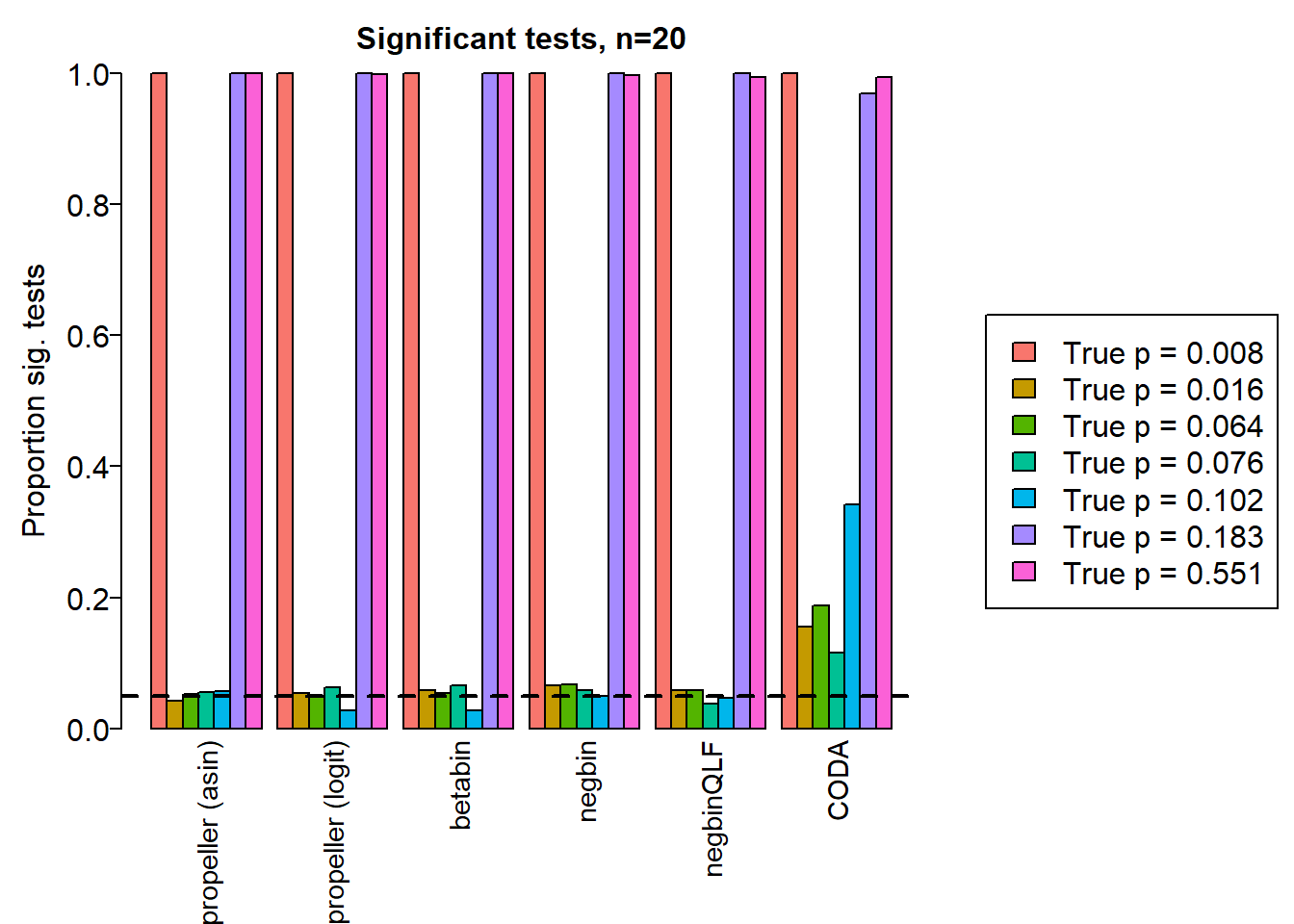

o <- order(trueprops)
mysig <- sig.disc[o,4:9]
colnames(mysig) <- names
pheatmap(mysig, scale="none", cluster_rows = FALSE, cluster_cols = FALSE,
         labels_row = c(expression(paste(pi, " = 0.008*", sep="")),
                        expression(paste(pi, " = 0.016", sep="")),
                        expression(paste(pi, " = 0.064", sep="")),
                        expression(paste(pi, " = 0.076", sep="")),
                        expression(paste(pi, " = 0.102", sep="")),
                        expression(paste(pi, " = 0.183*", sep="")),
                        expression(paste(pi, " = 0.551*", sep=""))),
         main=paste("Significant tests, n=",nsamp/2,sep=""))

sig.disc20 <- sig.disc

auc.asin <- auc.logit <- auc.bb <- auc.nb <- auc.qlf <- auc.coda <- rep(NA,nsim)
for(i in 1:nsim){
  auc.asin[i] <- auroc(score=1-pval.asin[,i],bool=de)
  auc.logit[i] <- auroc(score=1-pval.logit[,i],bool=de)
  auc.bb[i] <- auroc(score=1-pval.bb[,i],bool=de)
  auc.nb[i] <- auroc(score=1-pval.nb[,i],bool=de)
  auc.qlf[i] <- auroc(score=1-pval.qlf[,i],bool=de)
  auc.coda[i] <- auroc(score=1-pval.coda[,i],bool=de)
}

mean(auc.asin)

[1] 0.99975

mean(auc.logit)

[1] 0.9995

mean(auc.bb)

[1] 0.9995833

mean(auc.nb)

[1] 0.9985833

mean(auc.qlf)

[1] 0.9986667

mean(auc.coda)

[1] 0.9849167

auc.mat[4,1] <- mean(auc.asin)
auc.mat[4,2] <- mean(auc.logit)
auc.mat[4,3] <- mean(auc.bb)
auc.mat[4,4] <- mean(auc.nb)
auc.mat[4,5] <- mean(auc.qlf)
auc.mat[4,6] <- mean(auc.coda)

par(mfrow=c(1,1))
par(mar=c(9,5,3,2))
barplot(c(mean(auc.asin),mean(auc.logit),mean(auc.bb),mean(auc.nb),mean(auc.qlf),mean(auc.coda)), ylim=c(0,1), ylab= "AUC", cex.axis=1.5, cex.lab=1.5, names=names, las=2, cex.names = 1.5)
title(paste("AUC: sample size n=",nsamp/2,sep=""),cex.main=1.5)

save(sig.disc3, sig.disc5, sig.disc10, sig.disc20, auc.mat, names, trueprops,
     file="./output/TrueDiffSimResults.Rda")

Session information

sessionInfo()

R version 4.2.0 (2022-04-22 ucrt)
Platform: x86_64-w64-mingw32/x64 (64-bit)
Running under: Windows 10 x64 (build 22000)

Matrix products: default

locale:
[1] LC_COLLATE=English_United States.utf8 
[2] LC_CTYPE=English_United States.utf8   
[3] LC_MONETARY=English_United States.utf8
[4] LC_NUMERIC=C                          
[5] LC_TIME=English_United States.utf8    

attached base packages:
[1] stats     graphics  grDevices utils     datasets  methods   base     

other attached packages:
[1] gt_0.6.0        pheatmap_1.0.12 edgeR_3.38.1    limma_3.52.1   
[5] speckle_0.99.0  workflowr_1.7.0

loaded via a namespace (and not attached):
  [1] backports_1.4.1             plyr_1.8.7                 
  [3] igraph_1.3.1                lazyeval_0.2.2             
  [5] sp_1.4-7                    splines_4.2.0              
  [7] BiocParallel_1.30.2         listenv_0.8.0              
  [9] scattermore_0.8             GenomeInfoDb_1.32.2        
 [11] ggplot2_3.3.6               digest_0.6.29              
 [13] htmltools_0.5.2             fansi_1.0.3                
 [15] checkmate_2.1.0             magrittr_2.0.3             
 [17] memoise_2.0.1               tensor_1.5                 
 [19] cluster_2.1.3               ROCR_1.0-11                
 [21] globals_0.15.0              Biostrings_2.64.0          
 [23] matrixStats_0.62.0          spatstat.sparse_2.1-1      
 [25] colorspace_2.0-3            blob_1.2.3                 
 [27] ggrepel_0.9.1               xfun_0.31                  
 [29] dplyr_1.0.9                 callr_3.7.0                
 [31] crayon_1.5.1                RCurl_1.98-1.6             
 [33] jsonlite_1.8.0              org.Mm.eg.db_3.15.0        
 [35] progressr_0.10.0            spatstat.data_2.2-0        
 [37] survival_3.3-1              zoo_1.8-10                 
 [39] glue_1.6.2                  polyclip_1.10-0            
 [41] gtable_0.3.0                zlibbioc_1.42.0            
 [43] XVector_0.36.0              leiden_0.4.2               
 [45] DelayedArray_0.22.0         SingleCellExperiment_1.18.0
 [47] future.apply_1.9.0          BiocGenerics_0.42.0        
 [49] abind_1.4-5                 scales_1.2.0               
 [51] DBI_1.1.2                   spatstat.random_2.2-0      
 [53] miniUI_0.1.1.1              Rcpp_1.0.8.3               
 [55] viridisLite_0.4.0           xtable_1.8-4               
 [57] reticulate_1.25             spatstat.core_2.4-4        
 [59] bit_4.0.4                   stats4_4.2.0               
 [61] htmlwidgets_1.5.4           httr_1.4.3                 
 [63] RColorBrewer_1.1-3          ellipsis_0.3.2             
 [65] Seurat_4.1.1                ica_1.0-2                  
 [67] scuttle_1.6.2               pkgconfig_2.0.3            
 [69] uwot_0.1.11                 sass_0.4.1                 
 [71] deldir_1.0-6                locfit_1.5-9.5             
 [73] utf8_1.2.2                  tidyselect_1.1.2           
 [75] rlang_1.0.2                 reshape2_1.4.4             
 [77] later_1.3.0                 AnnotationDbi_1.58.0       
 [79] munsell_0.5.0               tools_4.2.0                
 [81] cachem_1.0.6                cli_3.3.0                  
 [83] generics_0.1.2              RSQLite_2.2.14             
 [85] ggridges_0.5.3              evaluate_0.15              
 [87] stringr_1.4.0               fastmap_1.1.0              
 [89] yaml_2.3.5                  goftest_1.2-3              
 [91] org.Hs.eg.db_3.15.0         processx_3.5.3             
 [93] knitr_1.39                  bit64_4.0.5                
 [95] fs_1.5.2                    fitdistrplus_1.1-8         
 [97] purrr_0.3.4                 RANN_2.6.1                 
 [99] KEGGREST_1.36.0             sparseMatrixStats_1.8.0    
[101] pbapply_1.5-0               future_1.26.1              
[103] nlme_3.1-157                whisker_0.4                
[105] mime_0.12                   compiler_4.2.0             
[107] rstudioapi_0.13             plotly_4.10.0              
[109] png_0.1-7                   spatstat.utils_2.3-1       
[111] tibble_3.1.7                bslib_0.3.1                
[113] stringi_1.7.6               highr_0.9                  
[115] ps_1.7.0                    rgeos_0.5-9                
[117] lattice_0.20-45             Matrix_1.4-1               
[119] vctrs_0.4.1                 pillar_1.7.0               
[121] lifecycle_1.0.1             spatstat.geom_2.4-0        
[123] lmtest_0.9-40               jquerylib_0.1.4            
[125] RcppAnnoy_0.0.19            data.table_1.14.2          
[127] cowplot_1.1.1               bitops_1.0-7               
[129] irlba_2.3.5                 GenomicRanges_1.48.0       
[131] httpuv_1.6.5                patchwork_1.1.1            
[133] R6_2.5.1                    promises_1.2.0.1           
[135] KernSmooth_2.23-20          gridExtra_2.3              
[137] IRanges_2.30.0              parallelly_1.31.1          
[139] codetools_0.2-18            MASS_7.3-57                
[141] assertthat_0.2.1            SummarizedExperiment_1.26.1
[143] rprojroot_2.0.3             SeuratObject_4.1.0         
[145] sctransform_0.3.3           S4Vectors_0.34.0           
[147] GenomeInfoDbData_1.2.8      mgcv_1.8-40                
[149] parallel_4.2.0              beachmat_2.12.0            
[151] rpart_4.1.16                grid_4.2.0                 
[153] tidyr_1.2.0                 DelayedMatrixStats_1.18.0  
[155] rmarkdown_2.14              MatrixGenerics_1.8.0       
[157] Rtsne_0.16                  git2r_0.30.1               
[159] getPass_0.2-2               Biobase_2.56.0             
[161] shiny_1.7.1