Data exploration: healthy human PBMCs
Belinda Phipson
31 May 2022
Last updated: 2022-06-01
Checks: 7 0
Knit directory: propeller-paper-analysis/
This reproducible R Markdown analysis was created with workflowr (version 1.7.0). The Checks tab describes the reproducibility checks that were applied when the results were created. The Past versions tab lists the development history.
Great! Since the R Markdown file has been committed to the Git repository, you know the exact version of the code that produced these results.
Great job! The global environment was empty. Objects defined in the global environment can affect the analysis in your R Markdown file in unknown ways. For reproduciblity it’s best to always run the code in an empty environment.
The command set.seed(20220531) was run prior to running
the code in the R Markdown file. Setting a seed ensures that any results
that rely on randomness, e.g. subsampling or permutations, are
reproducible.
Great job! Recording the operating system, R version, and package versions is critical for reproducibility.
Nice! There were no cached chunks for this analysis, so you can be confident that you successfully produced the results during this run.
Great job! Using relative paths to the files within your workflowr project makes it easier to run your code on other machines.
Great! You are using Git for version control. Tracking code development and connecting the code version to the results is critical for reproducibility.
The results in this page were generated with repository version ee88aa1. See the Past versions tab to see a history of the changes made to the R Markdown and HTML files.
Note that you need to be careful to ensure that all relevant files for
the analysis have been committed to Git prior to generating the results
(you can use wflow_publish or
wflow_git_commit). workflowr only checks the R Markdown
file, but you know if there are other scripts or data files that it
depends on. Below is the status of the Git repository when the results
were generated:
Ignored files:
    Ignored:    .Rproj.user/

Untracked files:
    Untracked:  data/CTpropsTransposed.txt
    Untracked:  data/CelltypeLevels.csv
    Untracked:  data/TypeIErrTables.Rdata
    Untracked:  data/appnote1cdata.rdata
    Untracked:  data/cold_warm_fresh_cellinfo.txt
    Untracked:  data/covid.cell.annotation.meta.txt
    Untracked:  data/heartFYA.Rds
    Untracked:  data/nullsimsVaryN_results.Rdata
    Untracked:  data/pool_1.rds
    Untracked:  data/sampleinfo.csv
    Untracked:  output/Fig1ab.pdf
    Untracked:  output/Fig1cde.pdf
Note that any generated files, e.g. HTML, png, CSS, etc., are not included in this status report because it is ok for generated content to have uncommitted changes.
These are the previous versions of the repository in which changes were
made to the R Markdown (analysis/pbmcJP.Rmd) and HTML
(docs/pbmcJP.html) files. If you’ve configured a remote Git
repository (see ?wflow_git_remote), click on the hyperlinks
in the table below to view the files as they were in that past version.
| File | Version | Author | Date | Message |
|---|---|---|---|---|
| Rmd | ee88aa1 | bphipson | 2022-06-01 | Add my first analysis |
Load the libraries
library(Seurat)
library(speckle)
library(limma)
library(ggplot2)
library(edgeR)
library(patchwork)
library(cowplot)
library(gridGraphics)set.seed(10)Read the data into R
The data is stored in a Seurat object. The cells have been classified into broader and more refined cell types.
pbmc <- readRDS("./data/pool_1.rds")Visualise the data by cell type and individual
# Cell type information
table(pbmc$predicted.celltype.l2)
            ASDC   B intermediate         B memory          B naive
               1              570              361              871
       CD14 Mono        CD16 Mono          CD4 CTL        CD4 Naive
             522              225              383             3552
         CD4 TCM          CD4 TEM        CD8 Naive          CD8 TCM
            3451              389              597              205
         CD8 TEM             cDC2              dnT            Eryth
            2421               20               43                5
             gdT             HSPC              ILC             MAIT
               4               18                5              189
              NK NK Proliferating    NK_CD56bright              pDC
            2582               43              134                7
     Plasmablast         Platelet             Treg
              10               27              414
DimPlot(pbmc, group.by = "predicted.celltype.l2")
table(pbmc$individual)
682_683 683_684 684_685 685_686 686_687 687_688 688_689 689_690 690_691 691_692
   1185    1478    1042    1613    1309    1486    1582    1789    1462    1505
692_693 693_694
   1310    1288
DimPlot(pbmc, group.by = "individual")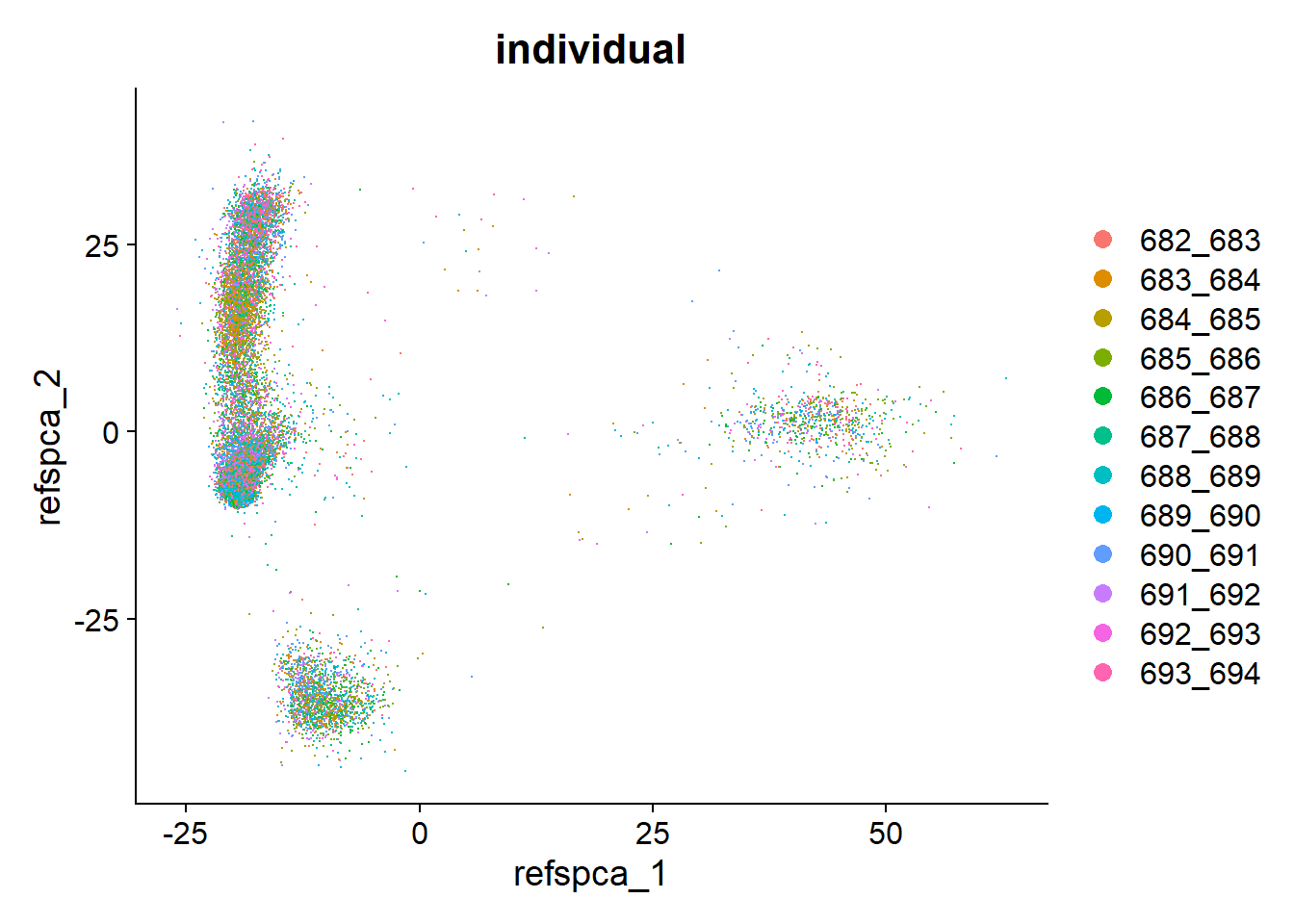
Run the Seurat workflow for normalisation, scaling, PCA and UMAP
pbmc <- NormalizeData(pbmc)
pbmc <- FindVariableFeatures(pbmc, selection.method = "vst", nfeatures = 2000)
pbmc <- ScaleData(pbmc)
pbmc <- RunPCA(pbmc, features = VariableFeatures(object = pbmc))
ElbowPlot(pbmc)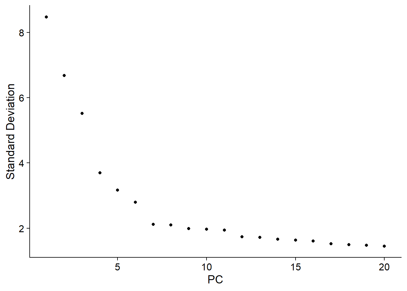
pbmc <- RunUMAP(pbmc, dims = 1:11)Visualise data with UMAP
DimPlot(pbmc, reduction = "umap",group.by = "predicted.celltype.l1", label=TRUE, label.size=6) + theme(legend.position = "none") + ggtitle("Broad cell type predictions")
DimPlot(pbmc, reduction = "umap",group.by = "predicted.celltype.l2") + ggtitle("Refined cell type predictions")
d1 <- DimPlot(pbmc, reduction = "umap",group.by = "predicted.celltype.l2") + theme(legend.position = "none") + ggtitle("a") + theme(plot.title = element_text(size = 18, hjust = 0))Explore cell type proportions among the 12 individuals
props <- getTransformedProps(clusters = pbmc$predicted.celltype.l2,
                             sample = pbmc$individual)

p1 <- plotCellTypeProps(clusters = pbmc$predicted.celltype.l2, sample = pbmc$individual) + theme(axis.text.x = element_text(angle = 45))+ ggtitle("Refined cell type proportions") +
theme(plot.title = element_text(size = 18, hjust = 0))
p1 + theme_bw() + theme(panel.grid.major = element_blank(),
                        panel.grid.minor = element_blank()) + theme(axis.text.x = element_text(angle = 45))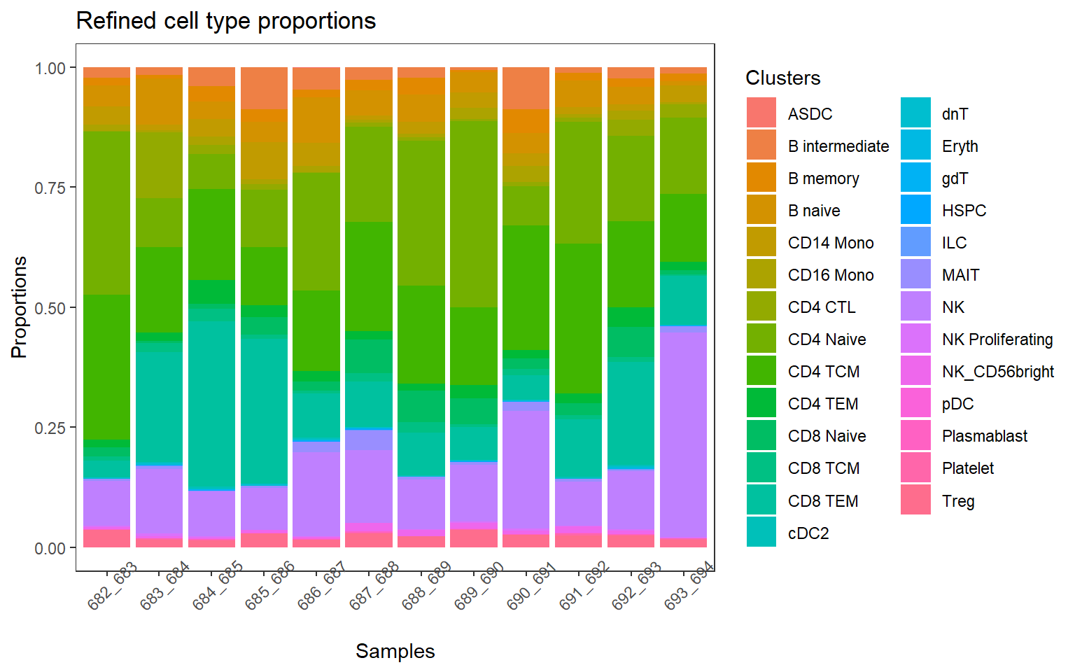
p2 <- plotCellTypeProps(clusters = pbmc$predicted.celltype.l1, sample = pbmc$individual)
p2 + theme(axis.text.x = element_text(angle = 45)) + ggtitle("Broad cell type proportions")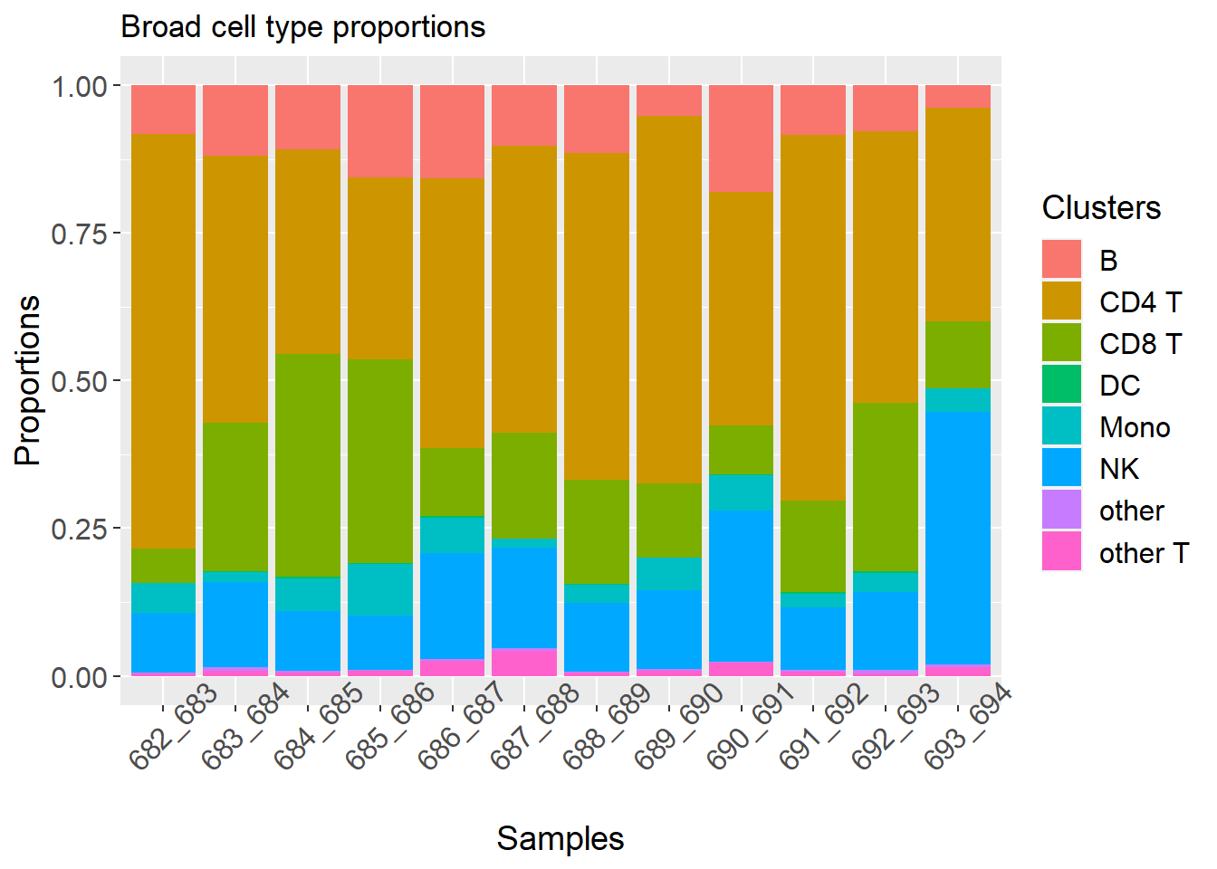
pdf(file="./output/Fig1ab.pdf", width =14, height=6)
d1 + p1
dev.off()
png
2 Exploring heterogeneity in cell type proportions between individuals
counts <- table(pbmc$predicted.celltype.l2, pbmc$individual)
baselineN <- rowSums(counts)
N <- sum(baselineN)
baselineprops <- baselineN/N
pbmc$final_ct <- factor(pbmc$predicted.celltype.l2, levels=names(sort(baselineprops, decreasing = TRUE)))counts <- table(pbmc$final_ct, pbmc$individual)
baselineN <- rowSums(counts)
N <- sum(baselineN)
baselineprops <- baselineN/Nprops <- getTransformedProps(clusters = pbmc$final_ct,
sample = pbmc$individual)cols <- ggplotColors(nrow(props$Proportions))
m <- match(rownames(props$Proportions),levels(factor(pbmc$predicted.celltype.l2)))par(mfrow=c(1,1))
par(mar=c(7,5,2,2))
plot(jitter(props$Proportions[,1]), col = cols[m], pch=16, ylim=c(0,max(props$Proportions)),
xaxt="n", xlab="", ylab="Cell type proportion", cex.lab=1.5, cex.axis=1.5)
for(i in 2:ncol(props$Proportions)){
points(jitter(1:nrow(props$Proportions)),props$Proportions[,i], col = cols[m],
pch=16)
}
axis(side=1, at=1:nrow(props$Proportions), las=2,
labels=rownames(props$Proportions))
title("Cell type proportions estimates for 12 individuals")
The mean-variance relationship plots below show that the data is overdispersed compared to what would be expected under a Binomial or Poisson distribution.
plotCellTypeMeanVar(counts)
plotCellTypePropsMeanVar(counts)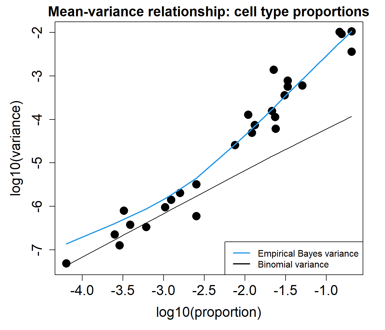
sessionInfo()R version 4.2.0 (2022-04-22 ucrt)
Platform: x86_64-w64-mingw32/x64 (64-bit)
Running under: Windows 10 x64 (build 22000)
Matrix products: default
locale:
[1] LC_COLLATE=English_United States.utf8
[2] LC_CTYPE=English_United States.utf8
[3] LC_MONETARY=English_United States.utf8
[4] LC_NUMERIC=C
[5] LC_TIME=English_United States.utf8
attached base packages:
[1] grid stats graphics grDevices utils datasets methods
[8] base
other attached packages:
[1] gridGraphics_0.5-1 cowplot_1.1.1 patchwork_1.1.1 edgeR_3.38.1
[5] ggplot2_3.3.6 limma_3.52.1 speckle_0.99.0 sp_1.4-7
[9] SeuratObject_4.1.0 Seurat_4.1.1 workflowr_1.7.0
loaded via a namespace (and not attached):
[1] utf8_1.2.2 reticulate_1.25
[3] tidyselect_1.1.2 RSQLite_2.2.14
[5] AnnotationDbi_1.58.0 htmlwidgets_1.5.4
[7] BiocParallel_1.30.2 Rtsne_0.16
[9] munsell_0.5.0 codetools_0.2-18
[11] ica_1.0-2 statmod_1.4.36
[13] future_1.26.1 miniUI_0.1.1.1
[15] withr_2.5.0 spatstat.random_2.2-0
[17] colorspace_2.0-3 progressr_0.10.0
[19] Biobase_2.56.0 highr_0.9
[21] knitr_1.39 rstudioapi_0.13
[23] stats4_4.2.0 SingleCellExperiment_1.18.0
[25] ROCR_1.0-11 tensor_1.5
[27] listenv_0.8.0 MatrixGenerics_1.8.0
[29] labeling_0.4.2 git2r_0.30.1
[31] GenomeInfoDbData_1.2.8 polyclip_1.10-0
[33] farver_2.1.0 bit64_4.0.5
[35] rprojroot_2.0.3 parallelly_1.31.1
[37] vctrs_0.4.1 generics_0.1.2
[39] xfun_0.31 R6_2.5.1
[41] GenomeInfoDb_1.32.2 locfit_1.5-9.5
[43] bitops_1.0-7 spatstat.utils_2.3-1
[45] cachem_1.0.6 DelayedArray_0.22.0
[47] assertthat_0.2.1 promises_1.2.0.1
[49] scales_1.2.0 rgeos_0.5-9
[51] gtable_0.3.0 beachmat_2.12.0
[53] org.Mm.eg.db_3.15.0 globals_0.15.0
[55] processx_3.5.3 goftest_1.2-3
[57] rlang_1.0.2 splines_4.2.0
[59] lazyeval_0.2.2 spatstat.geom_2.4-0
[61] yaml_2.3.5 reshape2_1.4.4
[63] abind_1.4-5 httpuv_1.6.5
[65] tools_4.2.0 ellipsis_0.3.2
[67] spatstat.core_2.4-4 jquerylib_0.1.4
[69] RColorBrewer_1.1-3 BiocGenerics_0.42.0
[71] ggridges_0.5.3 Rcpp_1.0.8.3
[73] plyr_1.8.7 sparseMatrixStats_1.8.0
[75] zlibbioc_1.42.0 purrr_0.3.4
[77] RCurl_1.98-1.6 ps_1.7.0
[79] rpart_4.1.16 deldir_1.0-6
[81] pbapply_1.5-0 S4Vectors_0.34.0
[83] zoo_1.8-10 SummarizedExperiment_1.26.1
[85] ggrepel_0.9.1 cluster_2.1.3
[87] fs_1.5.2 magrittr_2.0.3
[89] RSpectra_0.16-1 data.table_1.14.2
[91] scattermore_0.8 lmtest_0.9-40
[93] RANN_2.6.1 whisker_0.4
[95] fitdistrplus_1.1-8 matrixStats_0.62.0
[97] mime_0.12 evaluate_0.15
[99] xtable_1.8-4 IRanges_2.30.0
[101] gridExtra_2.3 compiler_4.2.0
[103] tibble_3.1.7 KernSmooth_2.23-20
[105] crayon_1.5.1 htmltools_0.5.2
[107] mgcv_1.8-40 later_1.3.0
[109] tidyr_1.2.0 lubridate_1.8.0
[111] DBI_1.1.2 MASS_7.3-57
[113] Matrix_1.4-1 cli_3.3.0
[115] parallel_4.2.0 igraph_1.3.1
[117] GenomicRanges_1.48.0 pkgconfig_2.0.3
[119] getPass_0.2-2 plotly_4.10.0
[121] scuttle_1.6.2 spatstat.sparse_2.1-1
[123] bslib_0.3.1 XVector_0.36.0
[125] stringr_1.4.0 callr_3.7.0
[127] digest_0.6.29 sctransform_0.3.3
[129] RcppAnnoy_0.0.19 spatstat.data_2.2-0
[131] Biostrings_2.64.0 rmarkdown_2.14
[133] leiden_0.4.2 uwot_0.1.11
[135] DelayedMatrixStats_1.18.0 shiny_1.7.1
[137] lifecycle_1.0.1 nlme_3.1-157
[139] jsonlite_1.8.0 viridisLite_0.4.0
[141] fansi_1.0.3 pillar_1.7.0
[143] lattice_0.20-45 KEGGREST_1.36.0
[145] fastmap_1.1.0 httr_1.4.3
[147] survival_3.3-1 glue_1.6.2
[149] png_0.1-7 bit_4.0.4
[151] stringi_1.7.6 sass_0.4.1
[153] blob_1.2.3 org.Hs.eg.db_3.15.0
[155] memoise_2.0.1 dplyr_1.0.9
[157] irlba_2.3.5 future.apply_1.9.0