Cosmx human liver cancer sample
Melody Jin
2026-02-18
library(jazzPanda)
library(SpatialExperiment)
library(Seurat)
library(ggplot2)
library(data.table)
library(dplyr)
library(tidyr)
library(glmnet)
library(caret)
library(ComplexUpset)
library(ggrepel)
library(gridExtra)
library(patchwork)
library(RColorBrewer)
library(limma)
library(here)
library(data.table)
library(xtable)
library(corrplot)
source(here("code/utils.R"))
Load data
This section loads the provided Seurat object and extracts per-cell metadata and transcript coordinates. We remove low-quality cells using QC flags, convert imaging pixel coordinates to millimetres per-field-of-view (FOV), and build a transcript-level table restricted to the liver cancer sample (slide_ID_numeric = 2). The coordinates are scaled to micrometres for plotting.
Load cell and transcript
data_nm  <- "cosmx_hlc"
seu <- readRDS(file.path(rdata$cosmx_data, "LiverDataReleaseSeurat_newUMAP.RDS"))


# local cell metadata
metadata <- as.data.frame(seu@meta.data)

## remove low quality cells
qc_cols <- c("qcFlagsRNACounts", "qcFlagsCellCounts", "qcFlagsCellPropNeg",
             "qcFlagsCellComplex", "qcFlagsCellArea","qcFlagsFOV")
metadata <- metadata[!apply(metadata[, qc_cols], 1, function(x) any(x == "Fail")), ]

cell_info_cols = c("x_FOV_px", "y_FOV_px", "x_slide_mm", "y_slide_mm",
                   "nCount_negprobes","nFeature_negprobes","nCount_falsecode",
                   "nFeature_falsecode","slide_ID_numeric", "Run_Tissue_name",
                   "fov","cellType","niche","cell_id")
cellCoords <- metadata[, cell_info_cols]

# keep cancer tissue only
liver_cancer = cellCoords[cellCoords$slide_ID_numeric==2 ,]

# load count matrix
counts <-seu[["RNA"]]@counts
cancer_cells = row.names(liver_cancer)

counts_cancer_sample = counts[, cancer_cells]

rm(counts)

dim(counts_cancer_sample)
[1] 1000 460169px_to_mm <- function(data){
all_fv = unique(data$fov)
parm_df = as.data.frame(matrix(0, ncol=5, nrow=length(all_fv)))
colnames(parm_df) = c("fov","y_slope","y_intcp","x_slope","x_intcp")
parm_df$fov = all_fv
for (fv in all_fv){
curr_fov = data[data$fov == fv, ]
curr_fov = curr_fov[order(curr_fov$x_FOV_px), ]
curr_fov = curr_fov[c(1, nrow(curr_fov)), ]
curr_fov = curr_fov[c(1,2),c("y_slide_mm","x_slide_mm","y_FOV_px","x_FOV_px") ]
# mm to px for y
y_slope = (curr_fov[2,"y_slide_mm"] - curr_fov[1,"y_slide_mm"]) / (curr_fov[2,"y_FOV_px"] - curr_fov[1,"y_FOV_px"])
y_intcp = curr_fov[2,"y_slide_mm"]- (y_slope*curr_fov[2,"y_FOV_px"])
# mm to px for x
x_slope = (curr_fov[2,"x_slide_mm"] - curr_fov[1,"x_slide_mm"]) / (curr_fov[2,"x_FOV_px"] - curr_fov[1,"x_FOV_px"])
x_intcp = curr_fov[2,"x_slide_mm"]- (x_slope*curr_fov[2,"x_FOV_px"])
parm_df[parm_df$fov==fv,"y_slope"] = y_slope
parm_df[parm_df$fov==fv,"y_intcp"] = y_intcp
parm_df[parm_df$fov==fv,"x_slope"] = x_slope
parm_df[parm_df$fov==fv,"x_intcp"] = x_intcp
}
return (parm_df)
}
# number of cells per fov
# all fovs contain at least 2 cells
fov_summary = as.data.frame(table(cellCoords[cellCoords$slide_ID_numeric==2,"fov"]))
# caculate the slope and intercept parameters for each fov
parm_df = px_to_mm(liver_cancer)
# convert px to mm for each cell based on the calculated params
liver_cancer <- liver_cancer %>%
left_join(parm_df, by = 'fov') %>%
mutate(
x_mm = x_FOV_px * x_slope + x_intcp,
y_mm = y_FOV_px * y_slope + y_intcp
) %>%
select(-x_slope, -y_slope, -x_intcp, -y_intcp)
transcriptCoords <-seu@misc$transcriptCoords
all_transcripts_cancer <- transcriptCoords[transcriptCoords$slideID == 2,]
# remove transctipt detections for low quality cells
all_transcripts_cancer <- all_transcripts_cancer[all_transcripts_cancer$cell_id %in% liver_cancer$cell_id, ]
ncells_tr = length(unique(all_transcripts_cancer$cell_id))
rm(transcriptCoords)
all_transcripts_cancer <- all_transcripts_cancer %>%
left_join(parm_df, by = 'fov') %>%
mutate(
x_mm = x_FOV_px * x_slope + x_intcp,
y_mm = y_FOV_px * y_slope + y_intcp
) %>%
select(-x_slope, -y_slope, -x_intcp, -y_intcp)
all_transcripts_cancer$x = all_transcripts_cancer$x_mm
all_transcripts_cancer$y = all_transcripts_cancer$y_mm
all_transcripts_cancer$feature_name = all_transcripts_cancer$target
hl_cancer = all_transcripts_cancer[,c("x","y","feature_name")]
all_genes = row.names(seu[["RNA"]]@counts)
rm(all_transcripts_cancer, seu)
hl_cancer$x = hl_cancer$x * 1000
hl_cancer$y = hl_cancer$y * 1000Quality assessment of negative controls
Negative probe
To evaluate nonspecific hybridization and potential technical artefacts, we examined the distribution of negative control probes (NegPrb*) across the dataset. These probes are not expected to hybridize with endogenous transcripts. Uniform low-level detection indicates well-controlled chemistry and minimal background noise.
The figure shows that NegPrb detections are relatively more abundant but uniformly distributed across the tissue, with no evidence of localized enrichment or clustering.
negprobes_coords <- hl_cancer[grepl("^NegPrb", hl_cancer$feature_name), ]

nc_tb = as.data.frame(sort(table(negprobes_coords$feature_name),
                           decreasing = TRUE))
colnames(nc_tb) = c("name","value_count")
negprobes_coords$feature_name =factor(negprobes_coords$feature_name,
                                      levels = nc_tb$name)

ggplot(nc_tb, aes(x = name, y = value_count)) +
    geom_bar(stat = "identity", color="white") +
    geom_text(aes(label = value_count),  vjust = -0.5, size = 3) +
    scale_y_continuous(expand = c(0,1), limits = c(0, 78000))+
    labs(title = " ", x = " ", y = "Number of total detections") +
    theme_bw()+
    theme(legend.position = "none",strip.background = element_rect(fill="white"),
          strip.text = element_text(size=8),
          axis.text.x= element_text(size=8, angle=90,vjust=0.5,hjust = 1),
          axis.title.y =element_text(size=8),
          axis.ticks=element_blank(),
          axis.title.x=element_blank(),
          panel.background=element_blank(),
          panel.grid.minor=element_blank(),
          plot.background=element_blank())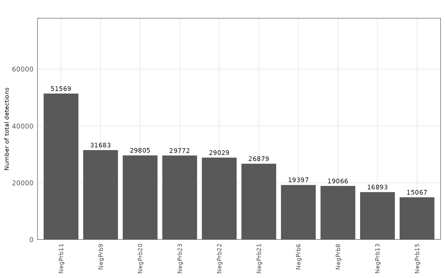
ggplot(negprobes_coords, aes(x=x, y=y))+
    geom_hex(bins=auto_hex_bin(nrow(negprobes_coords)))+
    theme_bw()+
    scale_fill_gradient(low="white", high="maroon4") +
    #facet_wrap(~feature_name, ncol=5)+
    ggtitle("Negprobes detections")+
    defined_theme+
    theme(legend.position = "top",aspect.ratio = 1/1,
          plot.title = element_text(size=rel(1.3)))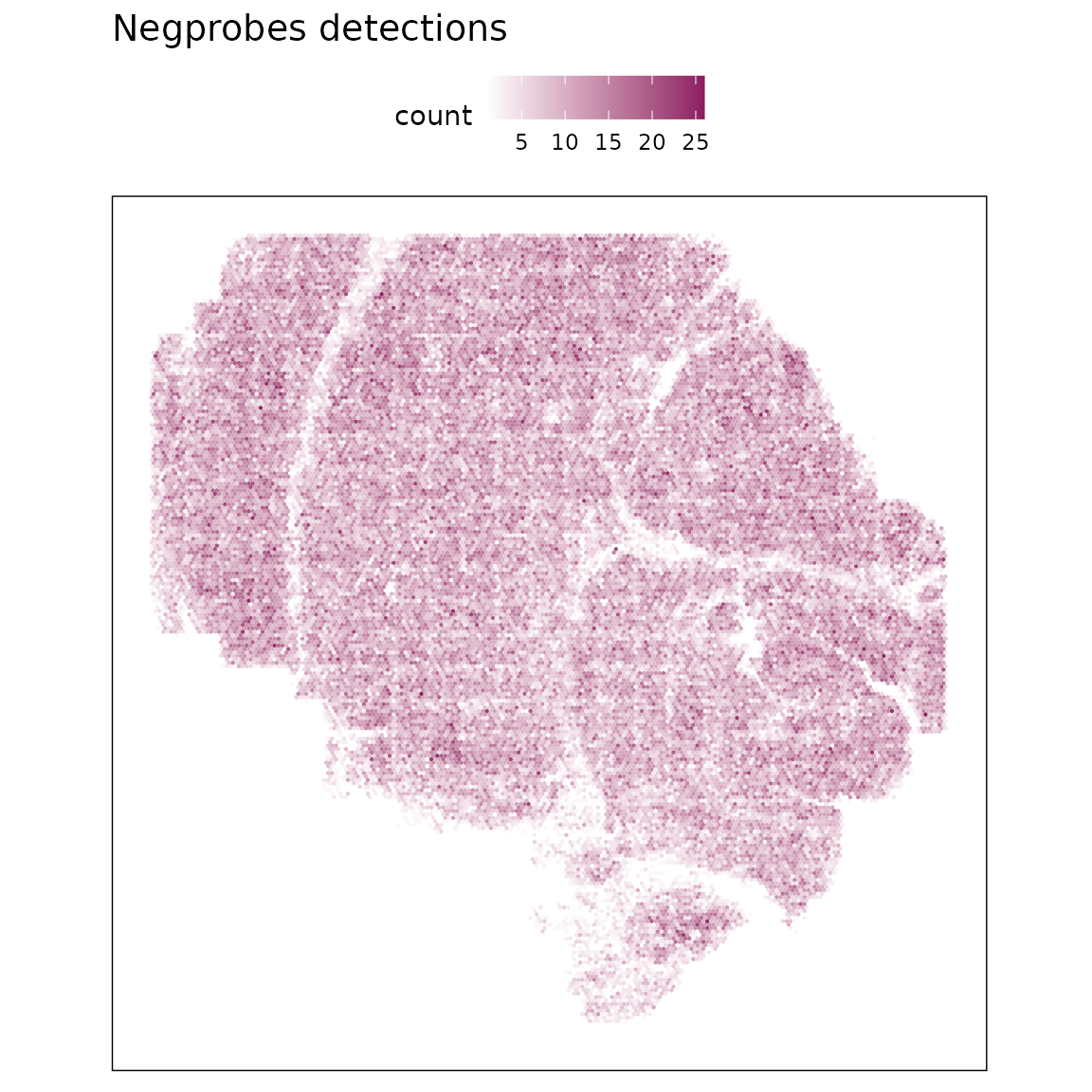
Falsecode probes
False-code probes are barcode sequences that do not match any real probes in the assay, serving as an estimate of background fluorescence and nonspecific binding. We visualized both the total detection counts per probe and their spatial distribution.
FalseCode features are detected at very low frequencies with no apparent spatial enrichment, indicating minimal false-positive signal.
falsecode_coords <- hl_cancer[grepl("^FalseCode", hl_cancer$feature_name), ]

fc_tb = as.data.frame(sort(table(falsecode_coords$feature_name), decreasing = TRUE))
colnames(fc_tb) = c("name","value_count")
fc_tb$cate = "total detection<1426"
fc_tb[fc_tb$value_count> 1426,"cate"] = "total detection>=1426"
fc_tb$cate=factor(fc_tb$cate,
                  levels=c("total detection<1426", "total detection>=1426"))
falsecode_coords$feature_name =factor(falsecode_coords$feature_name,
                                      levels = fc_tb$name)

ggplot(fc_tb, aes(x = name, y = value_count)) +
    geom_bar(stat = "identity",position = position_dodge(width = 0.9), color="white") +
    facet_wrap(~cate, ncol=1, scales = "free")+
    scale_y_continuous(expand = c(0,2))+
    labs(title = " ", x = " ", y = "Number of total detections") +
    theme_bw()+
    theme(legend.position = "none",strip.background = element_rect(fill="white"),
          strip.text = element_text(size=10),
          axis.text.x= element_text(size=10, angle=90,vjust=0.5,hjust = 1),
          axis.title.y =element_text(size=10),
          axis.ticks=element_blank(),
          axis.title.x=element_blank(),
          panel.background=element_blank(),
          panel.grid.minor=element_blank(),
          plot.background=element_blank())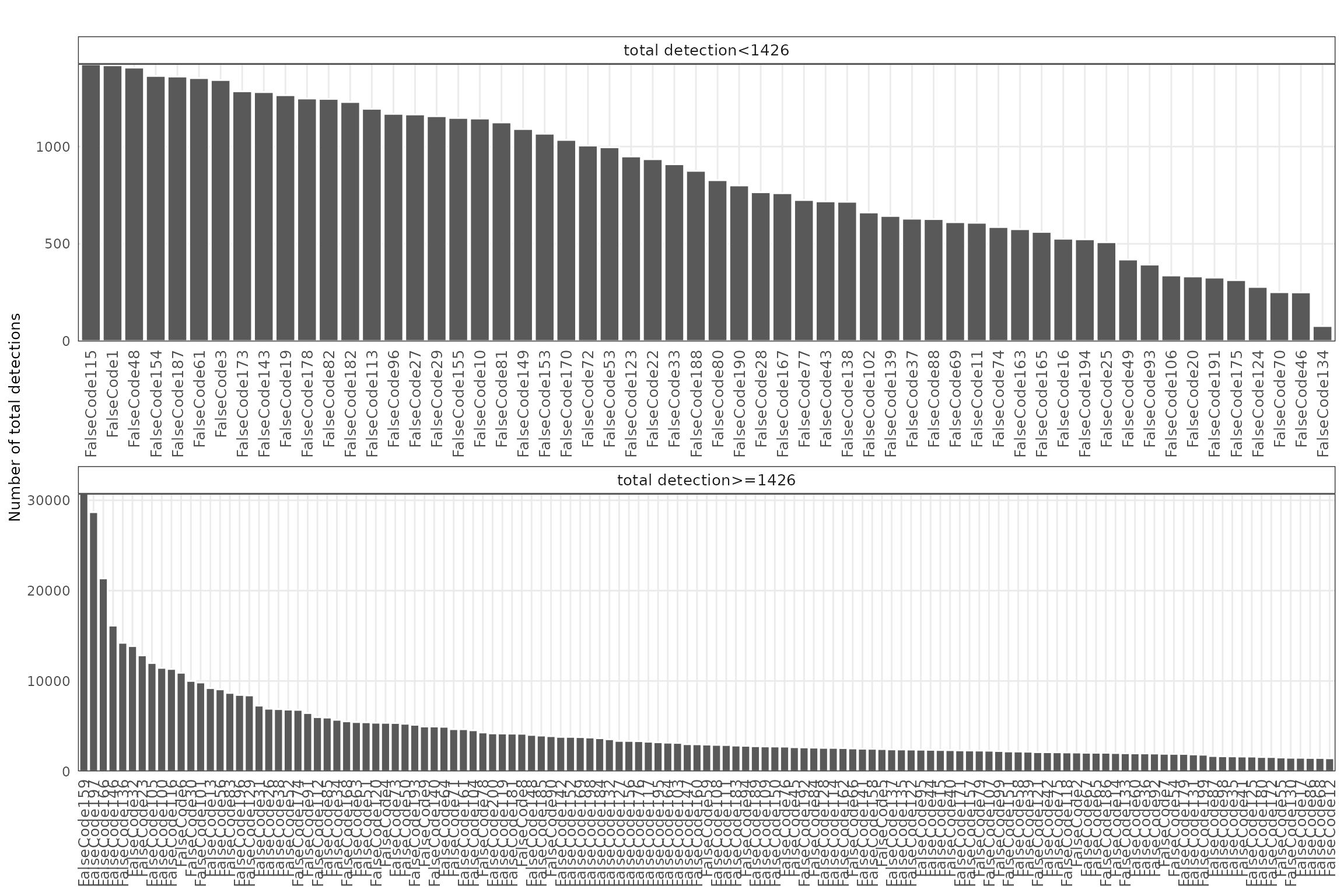
ggplot(falsecode_coords,aes(x=x, y=y))+
    geom_hex(bins=auto_hex_bin(nrow(falsecode_coords)))+
    scale_fill_gradient(low="white", high="maroon4") +
    theme_bw()+
    defined_theme+
    ggtitle("Falsecode detections")+
    theme(legend.position = "top",aspect.ratio = 1/1,
          plot.title = element_text(size=rel(1.3)))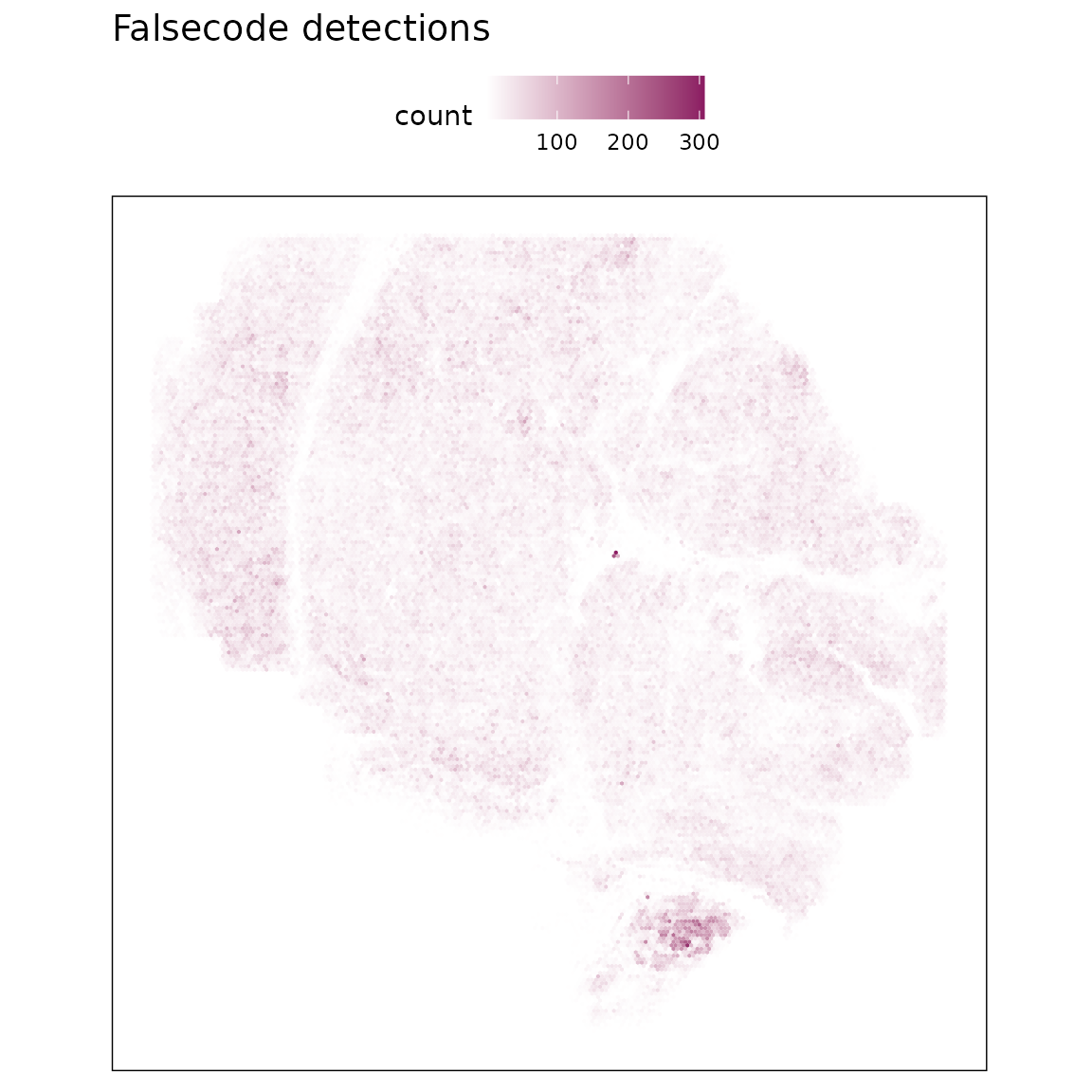
Single cell summary
These summary plots characterise per-cell detection counts and sparsity. We can calculate per-cell and per-gene summary statistics from the CosMx counts matrix:
Total detections per cell: sums all transcript counts in each cell.
Proportion of zeroes per cell: fraction of genes not detected in each cell.
Detected genes per cell: number of non-zero genes per cell.
Average expression per gene: mean expression across cells, ignoring zeros.
Each distribution is visualised with histograms and density curves to assess data quality and sparsity.
td_r1 <- colSums(counts_cancer_sample)
summary(td_r1)
Min. 1st Qu. Median Mean 3rd Qu. Max.
20 245 561 1036 1373 27422 pz_r1 <-colMeans(counts_cancer_sample==0)
summary(pz_r1) Min. 1st Qu. Median Mean 3rd Qu. Max.
0.053 0.698 0.811 0.781 0.879 0.995 numgene_r1 <- colSums(counts_cancer_sample!=0)
summary(numgene_r1) Min. 1st Qu. Median Mean 3rd Qu. Max.
5 121 189 219 302 947 td_df = as.data.frame(cbind(as.vector(td_r1),
rep("hliver_cancer", length(td_r1))))
colnames(td_df) = c("td","sample")
td_df$td= as.numeric(td_df$td)
# Build the entire summary as one string
output <- paste0(
"\n================= Summary Statistics =================\n\n",
"--- CosMx human liver cancer sample---\n",
make_sc_summary(td_r1, "Total detections per cell:"),
make_sc_summary(pz_r1, "Proportion of zeroes per cell:"),
make_sc_summary(numgene_r1, "Detected genes per cell:"),
"\n========================================================\n"
)
cat(output)
================= Summary Statistics =================

--- CosMx human liver cancer sample---
Total detections per cell:
  Min: 20.0000 |  1Q: 245.0000 |  Median: 561.0000 |  Mean: 1035.8867 |  3Q: 1373.0000 |  Max: 27422.0000
Proportion of zeroes per cell:
  Min: 0.0530 |  1Q: 0.6980 |  Median: 0.8110 |  Mean: 0.7809 |  3Q: 0.8790 |  Max: 0.9950
Detected genes per cell:
  Min: 5.0000 |  1Q: 121.0000 |  Median: 189.0000 |  Mean: 219.1153 |  3Q: 302.0000 |  Max: 947.0000

========================================================
p1<-ggplot(data = td_df, aes(x = td, color=sample)) +
geom_histogram(aes(y = after_stat(density)),
binwidth = 300, fill = "gray", color = "black") +
geom_density(color = "steelblue", size = 2) +
labs(title = "Distribution of total detections per cell",
x = " ", y = "Density") +
theme_minimal() +
theme(plot.title = element_text(hjust = 0.5),
strip.text = element_text(size=12))
pz = as.data.frame(cbind(as.vector(pz_r1),rep("hliver_cancer", length(pz_r1))))
colnames(pz) = c("prop_ze","sample")
pz$prop_ze= as.numeric(pz$prop_ze)
p2<-ggplot(data = pz, aes(x = prop_ze)) +
geom_histogram(aes(y = after_stat(density)),
binwidth = 0.05, fill = "gray", color = "black") +
geom_density(color = "steelblue", size = 2) +
labs(title = "Distribution of proportion of zeroes per cell",
x = " ", y = "Density") +
theme_minimal() +
theme(plot.title = element_text(hjust = 0.5),
strip.text = element_text(size=12))
numgens = as.data.frame(cbind(as.vector(numgene_r1),rep("hliver_cancer", length(numgene_r1))))
colnames(numgens) = c("numgen","sample")
numgens$numgen= as.numeric(numgens$numgen)
p3<-ggplot(data = numgens, aes(x = numgen)) +
geom_histogram(aes(y = after_stat(density)),
binwidth = 20, fill = "gray", color = "black") +
geom_density(color = "steelblue", size = 2) +
labs(title = "Distribution of detected genes per cell",
x = " ", y = "Density") +
theme_minimal() +
theme(plot.title = element_text(hjust = 0.5),
strip.text = element_text(size=12))cm_new1=counts_cancer_sample
cm_new1[cm_new1==0] = NA
cm_new1 = as.data.frame(cm_new1)
cm_new1$avg2 = rowMeans(cm_new1,na.rm = TRUE)
summary(cm_new1$avg2) Min. 1st Qu. Median Mean 3rd Qu. Max.
1.05 1.13 1.22 2.22 1.62 94.55 avg_exp = as.data.frame(cbind("avg"=cm_new1$avg2,
"sample"=rep("hliver_heathy", nrow(cm_new1))))
avg_exp$avg=as.numeric(avg_exp$avg)
p4<-ggplot(data = avg_exp, aes(x = avg, color=sample)) +
geom_histogram(aes(y = after_stat(density)),
binwidth = 0.5, fill = "gray", color = "black") +
geom_density(color = "orange", linewidth = 1) +
labs(title = "Distribution of average gene expression per cell",
x = " ", y = "Density") +
theme_minimal() +
theme(plot.title = element_text(hjust = 0.5),
strip.text = element_text(size=12))
layout_design <- (p1|p2)/(p3|p4)
print(layout_design)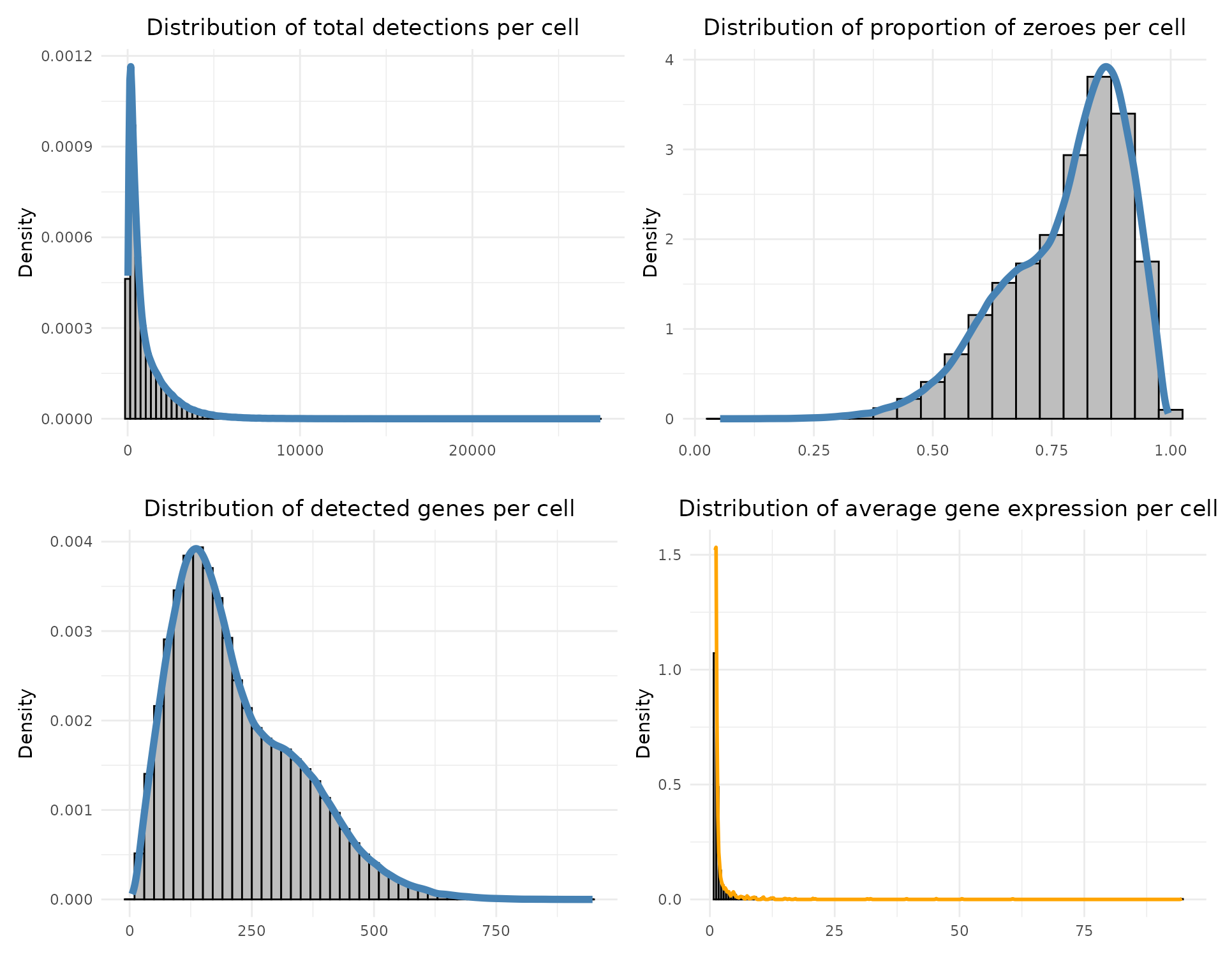
The total detection and mean expression distributions are right-skewed, indicating a majority of cells with modest transcript counts and a minority with high expression, as expected for spatial transcriptomics data. The high fraction of zero values per cell (peaking around 80–90%) reflects sparsity in subcellular-resolution assays.The median number of detected genes is around 561 for this cancer liver sample.
Refine clustering
The following code subsets to the liver cancer tissue section and harmonizes related cell subtypes into broader annotations (e.g., multiple macrophage and T-cell subtypes merged into “Macrophages” and “T”). The resulting coordinates are scaled and plotted using hexbin density maps, showing the spatial distribution of each annotated cell type across the tissue.
selected_cols = c("x_FOV_px", "y_FOV_px","x_slide_mm", "y_slide_mm", "slide_ID_numeric", "Run_Tissue_name", "fov","cellType","niche","cell_id" )
cluster_info = cellCoords[cellCoords$slide_ID_numeric=="2" & (row.names(cellCoords) %in% row.names(metadata)),selected_cols ]

colnames(cluster_info) =c("x_FOV_px","y_FOV_px" , "x", "y", "slide_ID_numeric", "Run_Tissue_name", "fov","cellTypes","niche","cell_id")
cluster_info$anno = as.character(cluster_info$cellTypes)
cluster_info[cluster_info$cellTypes %in% c("Antibody.secreting.B.cells", "Mature.B.cells"),"anno"] = "B"
cluster_info[cluster_info$cellTypes %in% c("CD3+.alpha.beta.T.cells", "gamma.delta.T.cells.1"),"anno"] = "T"
cluster_info[cluster_info$cellTypes %in% c("Non.inflammatory.macrophages", "Inflammatory.macrophages"),"anno"] = "Macrophages"

ig_clusters = c("NotDet")

cluster_info = cluster_info[cluster_info$anno != "NotDet",]

cluster_info$anno = factor(cluster_info$anno,
                            levels=c("tumor_1","tumor_2","Macrophages","T",
                                     "Periportal.LSECs","Stellate.cells","B",
                                     "Central.venous.LSECs","Cholangiocytes","Hep",
                                     "Portal.endothelial.cells",
                                     "NK.like.cells","Erthyroid.cells"))
cluster_info$cluster = cluster_info$anno
cluster_info$sample = "cancer"

cluster_info = cluster_info[!duplicated(cluster_info[,c("x","y")]),]
cluster_info$x = cluster_info$x * 1000
cluster_info$y = cluster_info$y * 1000


cluster_names = c("tumor_1","tumor_2","Macrophages",
                  "T", "Periportal.LSECs","Stellate.cells",
                  "B","Central.venous.LSECs","Cholangiocytes",
                  "Hep","Portal.endothelial.cells","NK.like.cells",
                  "Erthyroid.cells")

saveRDS(cluster_info, here(gdata,paste0(data_nm, "_clusters.Rds")))
# load generated data (see code above for how they were created)
cluster_info = readRDS(here(gdata,paste0(data_nm, "_clusters.Rds")))
cluster_info$anno_name = cluster_info$cluster
cluster_names = c("tumor_1","tumor_2","Macrophages",
"T", "Periportal.LSECs","Stellate.cells",
"B","Central.venous.LSECs","Cholangiocytes",
"Hep","Portal.endothelial.cells","NK.like.cells",
"Erthyroid.cells")
cluster_info$cluster = factor(cluster_info$cluster,
levels=cluster_names)
cluster_info$anno_name = factor(cluster_info$anno_name,
levels=cluster_names)
cluster_info = cluster_info[order(cluster_info$anno_name), ]
fig_ratio = cluster_info %>%
group_by(sample) %>%
summarise(
x_range = diff(range(x, na.rm = TRUE)),
y_range = diff(range(y, na.rm = TRUE)),
ratio = y_range / x_range,
.groups = "drop"
) %>% summarise(max_ratio = max(ratio)) %>% pull(max_ratio)We visualized the spatial distribution of annotated cell types to examine tissue structure and cell localization patterns in the CosMx liver cancer sample. The following plot displays all cells colored by their assigned cell type, highlighting the overall organization of the tissue.
ggplot(data = cluster_info,
        aes(x = x, y = y, color=cluster))+
        geom_point(size=0.0001)+
        facet_wrap(~sample)+
        theme_classic()+
        guides(color=guide_legend(title="", nrow = 4,
        override.aes=list(alpha=1, size=4)))+
        defined_theme+
        theme(aspect.ratio = fig_ratio,
              legend.position = "bottom",
              strip.text = element_blank())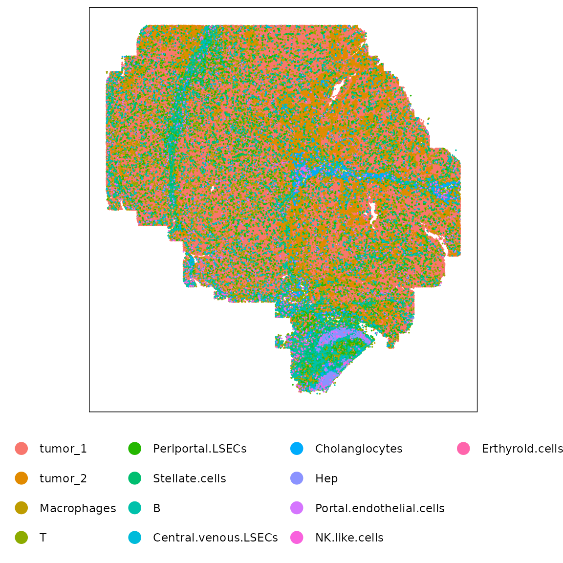
The faceted hexbin plots reveal that major cell types occupy distinct and spatially coherent regions within the section. Tumor regions (tumor_1, tumor_2) form dense contiguous areas, while immune and stromal populations such as macrophages, T cells, and periportal LSECs localize to the tissue periphery or vascular interfaces. Hepatocytes and cholangiocytes appear in spatially restricted niches consistent with expected hepatic zonation.
ggplot(data = cluster_info,
        aes(x = x, y = y))+
        geom_hex(bins = 200)+
        facet_wrap(~cluster, nrow=3)+
        scale_fill_gradient(low="white", high="maroon4") +
        theme_classic()+
        guides(color=guide_legend(title="",
                                  override.aes=list(alpha=1, size=8)))+
        defined_theme+
        theme(legend.position = "right",
              aspect.ratio = fig_ratio,
              strip.text = element_text(size=12))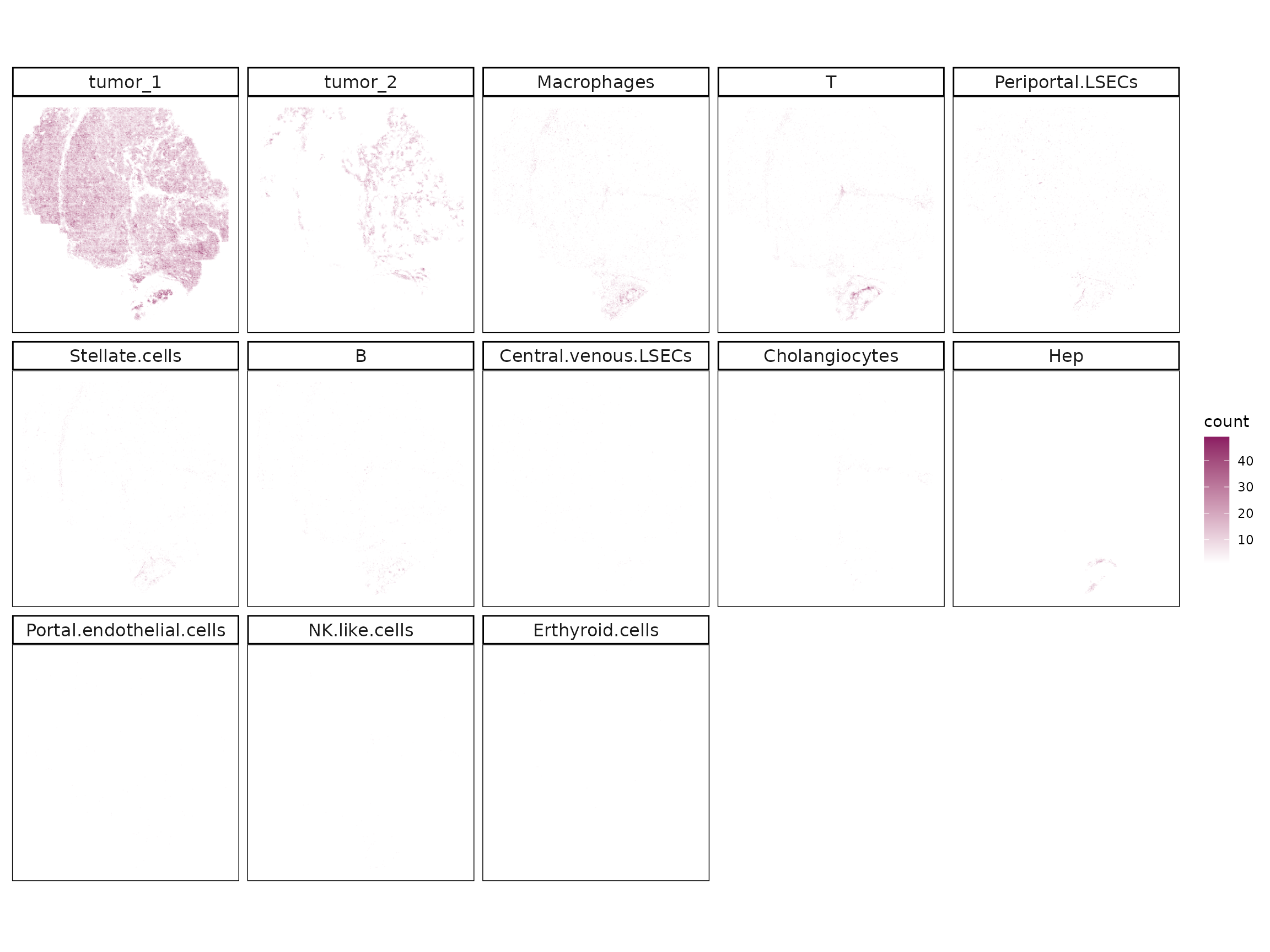
We quantified the number of cells assigned to each annotated cell type to assess the overall cellular composition of the CosMx liver cancer sample. The bar plot shows that tumor-associated cells (tumor_1 and tumor_2) overwhelmingly dominate the dataset, reflecting the high tumor cell density captured in this section. Among non-tumor populations, macrophages and T cells are the most prevalent, indicating notable immune infiltration within the tumor microenvironment. Stromal and endothelial subsets such as stellate cells, LSECs, and B cells are less abundant, while hepatocytes and cholangiocytes are relatively rare.
sum_df <- as.data.frame(table(cluster_info$anno_name))
colnames(sum_df) = c("cellType","n")
ggplot(sum_df, aes(x = cellType, y = n, fill=n)) +
    geom_bar(stat = "identity", position="stack", fill="black") +
    geom_text(aes(label = n),size=3,
              position = position_dodge(width = 0.9), vjust = -0.5) +
   scale_y_continuous(expand = c(0,1), limits=c(0,400000))+
    labs(title = " ", x = " ", y = "number of cells", fill="cell type") +
    theme_bw()+
    theme(legend.position = "none",
          axis.text= element_text(size=12, angle=90,vjust=0.5,hjust = 1),
          strip.text = element_text(size = rel(1.1)),
          axis.line=element_blank(),
          axis.text.y=element_blank(),axis.ticks=element_blank(),
          axis.title=element_text(size=12),
          panel.background=element_blank(),
          panel.grid.major=element_blank(),
          panel.grid.minor=element_blank(),
          plot.background=element_blank())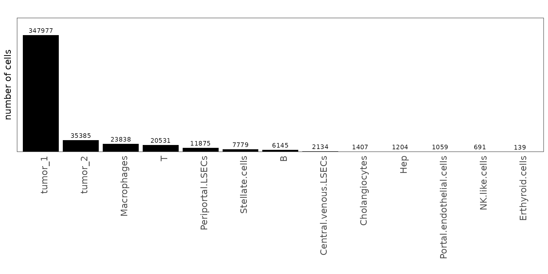
Detect marker genes
jazzPanda
We applied jazzPanda to this dataset using both the linear modelling and correlation-based approaches to detect spatially enriched marker genes across clusters.
Linear modelling approach
We first used the linear modelling approach to identify spatially enriched marker genes. The dataset was converted into spatial gene and cluster vectors using a 40 × 40 square binning strategy. False-code and negative-probe transcripts were included as background controls. For each gene, a linear model was fitted to estimate its spatial association with relevant cell type patterns.
grid_length = 40
seed_number=589
set.seed(seed_number)

hliver_vector_lst = get_vectors(x= list("cancer" = hl_cancer),
                                sample_names = "cancer",
                                cluster_info = cluster_info,
                                bin_type="square",
                                bin_param=c(grid_length, grid_length),
                                test_genes = all_genes,
                                n_cores =5)

falsecode_coords$sample = "cancer"
negprobes_coords$sample = "cancer"
kpt_cols = c("x","y","feature_name","sample")

nc_coords = rbind(falsecode_coords[,kpt_cols],negprobes_coords[,kpt_cols])

falsecode_names = unique(falsecode_coords$feature_name)
negprobe_names = unique(negprobes_coords$feature_name)
nc_vectors = create_genesets(x=list("cancer" = nc_coords),
                             sample_names=c("cancer"),
                             name_lst=list(falsecode=falsecode_names,
                                           negprobe=negprobe_names),
                             bin_type="square",
                             bin_param=c(grid_length, grid_length),
                             cluster_info=NULL)
set.seed(589)

jazzPanda_res_lst = lasso_markers(gene_mt=hliver_vector_lst$gene_mt,
                                  cluster_mt = hliver_vector_lst$cluster_mt,
                                  sample_names=c("cancer"),
                                  keep_positive=TRUE,
                                  background=nc_vectors,
                                  n_fold = 10)


saveRDS(hliver_vector_lst, here(gdata,paste0(data_nm, "_sq40_vector_lst.Rds")))
saveRDS(jazzPanda_res_lst, here(gdata,paste0(data_nm, "_jazzPanda_res_lst.Rds")))
We then used get_top_mg to extract unique marker genes
for each cluster based on a coefficient cutoff of 0.1. This function
returns the top spatially enriched genes that are most specific to each
cluster. In contrast, if shared marker genes across clusters are of
interest, all significant genes can be retrieved using
get_full_mg.
# load from saved objects
jazzPanda_res_lst = readRDS(here(gdata,paste0(data_nm, "_jazzPanda_res_lst.Rds")))
sv_lst = readRDS(here(gdata,paste0(data_nm, "_sq40_vector_lst.Rds")))
nbins = 1600
jazzPanda_res = get_top_mg(jazzPanda_res_lst, coef_cutoff=0.1)


seu = readRDS(here(gdata,paste0(data_nm, "_seu.Rds")))
seu <- subset(seu, cells = cluster_info$cell_id)
Idents(seu)=cluster_info$anno_name[match(colnames(seu), cluster_info$cell_id)]
seu$sample = cluster_info$sample[match(colnames(seu), cluster_info$cell_id)]
Idents(seu) = factor(Idents(seu), levels = cluster_names)
Cluster to cluster correlation
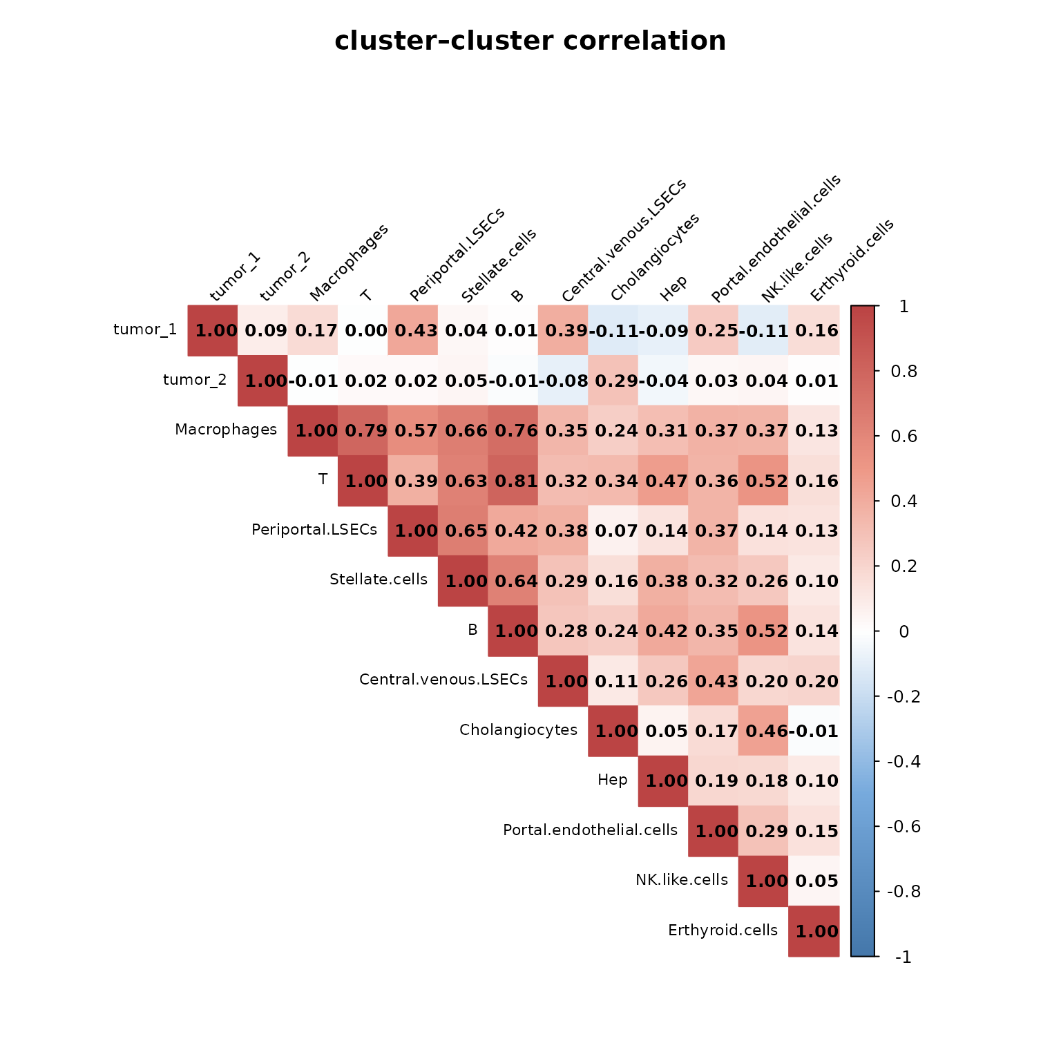
To examine the relationship between spatial expression patterns of different cell types, we computed pairwise Pearson correlations between the cluster-level vectors generated by jazzPanda. The resulting correlation matrix (visualized above) reflects how similar the spatial gene expression signatures are across annotated clusters.
The figure shows strong positive correlations among stromal and immune populations, particularly between macrophages, T cells, and periportal LSECs, suggesting coordinated spatial localization or shared microenvironmental influence. Tumor clusters (tumor_1, tumor_2) display moderate correlations with macrophages and LSECs, consistent with tumor–stroma and tumor–immune interactions. In contrast, hepatocytes and cholangiocytes exhibit weak or negative correlations with most other clusters, reflecting their distinct transcriptional and spatial niches.
cluster_mtt = sv_lst$cluster_mt
cluster_mtt = cluster_mtt[,cluster_names]
cor_M_cluster = cor(cluster_mtt,cluster_mtt,method = "pearson")
col <- colorRampPalette(c("#4477AA", "#77AADD", "#FFFFFF","#EE9988", "#BB4444"))
corrplot(
  cor_M_cluster,
  method      = "color",
  col         = col(200),
  diag        = TRUE,
  addCoef.col = "black",
  type        = "upper",
  tl.col      = "black",
  tl.cex      = 0.7,
  number.cex  = 0.8,
  tl.srt      = 45,
  mar         = c(0, 0, 3, 0),
  sig.level   = 0.05,
  insig       = "blank",
  title       = "cluster–cluster correlation",
  cex.main    = 1.2
)
The dot plot displays the top 10 marker genes identified by the jazzPanda linear modelling approach across annotated cell types. Dot size represents the proportion of cells expressing each gene, and color indicates average expression level. The figure shows cell-type-specific expression patterns—tumor clusters enriched for metabolic and stress-response genes, macrophages for immune and phagocytic genes, stellate cells for extracellular matrix components, and hepatocytes for classic liver-function markers.
glm_mg = jazzPanda_res[jazzPanda_res$top_cluster != "NoSig", ]
glm_mg$top_cluster = factor(glm_mg$top_cluster, levels = cluster_names)
top_mg_glm <- glm_mg %>%
  group_by(top_cluster) %>%
  arrange(desc(glm_coef), .by_group = TRUE) %>%
  slice_max(order_by = glm_coef, n = 10) %>%
  select(top_cluster, gene, glm_coef)

p1<-DotPlot(seu, features = top_mg_glm$gene) +
     scale_colour_gradient(low = "white", high = "red") +
    coord_flip()+
    theme(axis.text.x = element_text(angle = 45, hjust = 1, vjust = 1))+
    labs(title = "Top 10 marker genes (jazzPanda-glm)", x="", y="")

p1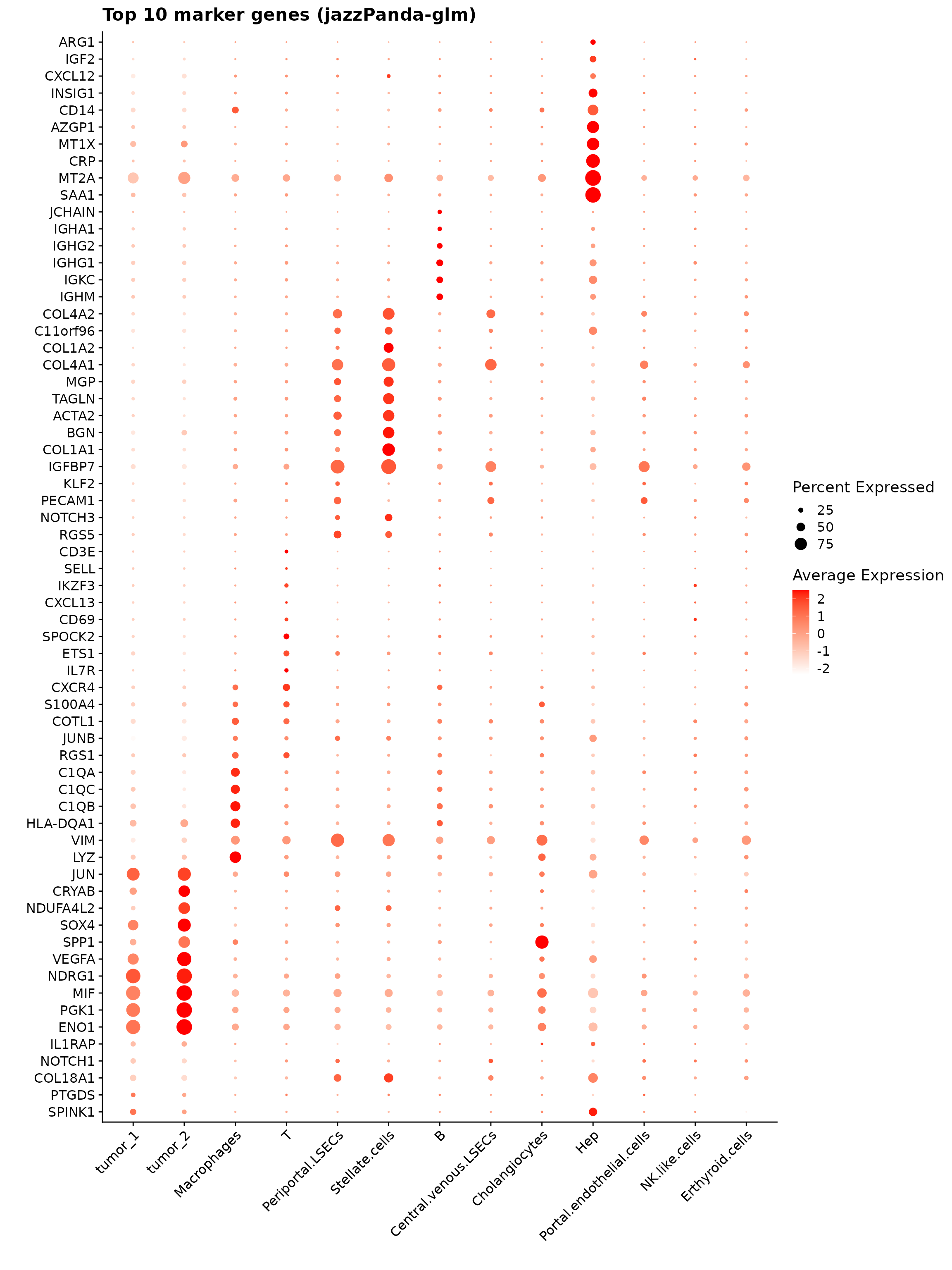
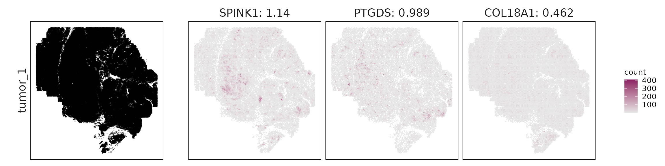
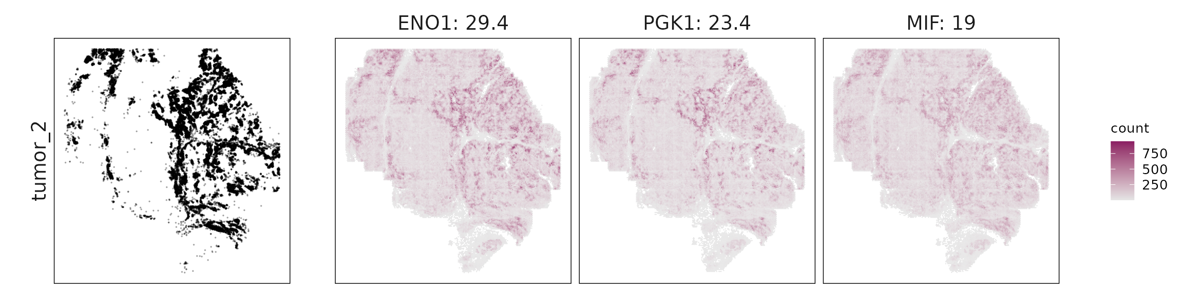
Top3 marker genes by jazzPanda_glm
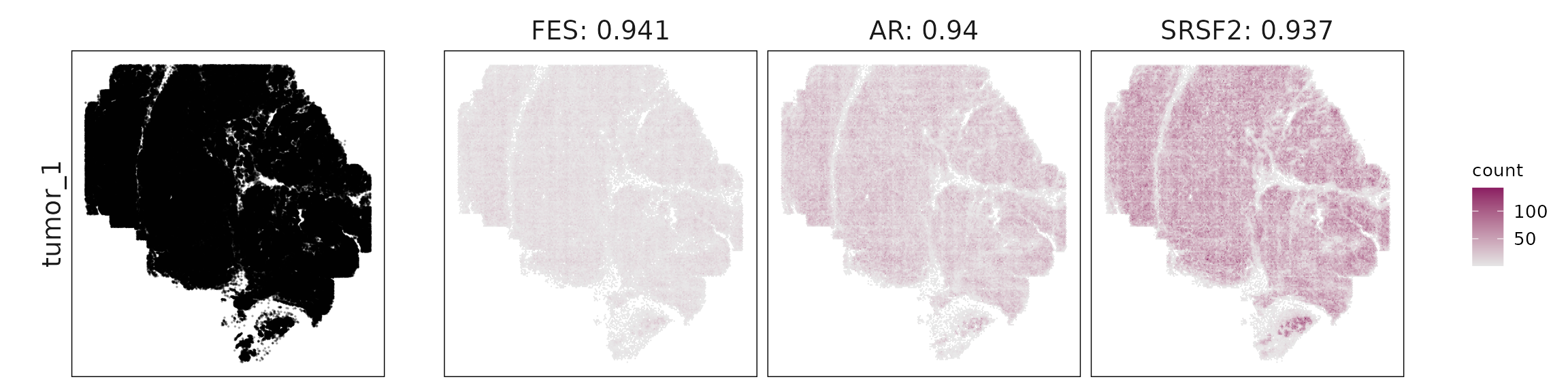
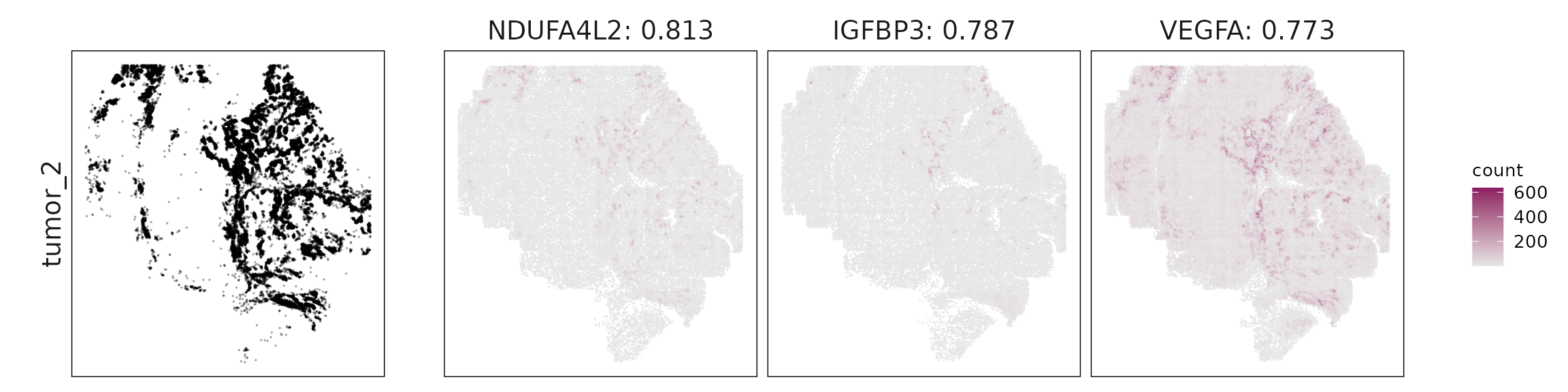
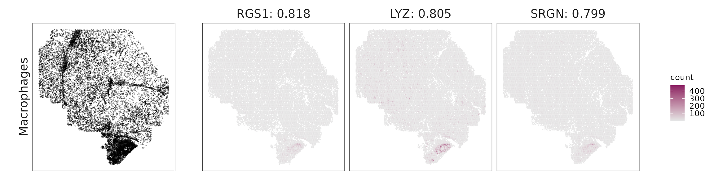
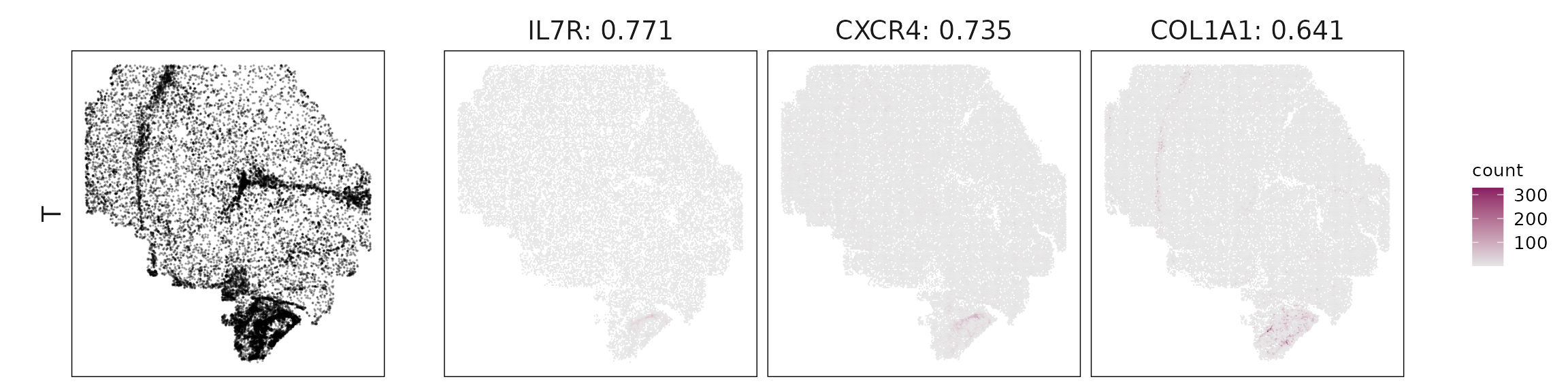
We visualized the top three marker genes identified by the linear modelling approach for each cluster. For each selected gene, its spatial transcript locations were plotted alongside the corresponding cluster map. Across clusters, the spatial expression patterns of marker genes closely match the distribution of their associated cell types
for (cl in cluster_names){
    inters=jazzPanda_res[jazzPanda_res$top_cluster==cl,"gene"]
    rounded_val=signif(as.numeric(jazzPanda_res[inters,"glm_coef"]),
                          digits = 3)
    inters_df = as.data.frame(cbind(gene=inters, value=rounded_val))
    inters_df$value = as.numeric(inters_df$value)
    inters_df=inters_df[order(inters_df$value, decreasing = TRUE),]
    inters_df$text= paste(inters_df$gene,inters_df$value,sep=": ")

    if (length(inters > 0)){
        inters_df = inters_df[1:min(3, nrow(inters_df)),]
        inters = inters_df$gene
        iters_sp1= hl_cancer$feature_name %in% inters
        vis_r1 =hl_cancer[iters_sp1,
                        c("x","y","feature_name")]
        vis_r1$value = inters_df[match(vis_r1$feature_name,inters_df$gene),
                        "value"]
        vis_r1=vis_r1[order(vis_r1$value,decreasing = TRUE),]
        vis_r1$text_label= paste(vis_r1$feature_name,
                            vis_r1$value,sep=": ")
        vis_r1$text_label=factor(vis_r1$text_label, levels=inters_df$text)

        vis_r1 = vis_r1[order(vis_r1$text_label),]

        genes_plt <- plot_top3_genes(vis_df=vis_r1, fig_ratio=fig_ratio)

        cluster_data =  cluster_info[cluster_info$cluster==cl, ]
        cl_pt<- ggplot(data =cluster_data,
                    aes(x = x, y = y, color=sample))+
                    geom_point(size=0.001, alpha=0.3)+
                    facet_wrap(~anno_name, nrow=1,strip.position = "left")+
                    scale_color_manual(values = c("black"))+
                    defined_theme +
                theme(legend.position = "none",
                        aspect.ratio = fig_ratio,
                        strip.background = element_blank(),
                        plot.margin = margin(0, 0, 0, 0),
                        legend.key.width = unit(15, "cm"),
                        strip.text = element_text(size = rel(1.3)))

        layout_design <- (wrap_plots(cl_pt, ncol = 1) | genes_plt) +
            plot_layout(widths = c(1, 3), heights = c(1))

        print(layout_design)

    }
  }
Cluster vector versus marker gene vector
We examined the relationship between each cluster vector and its top three marker gene vectors identified by the linear modelling approach. Each scatter plot compares the spatial activation strength of a marker gene with the corresponding cluster vector across spatial bins.
For most clusters, marker genes show a strong positive trend with the corresponding cluster vector, confirming that their expression is spatially aligned with the inferred cluster domain.
However, several genes (e.g. ENO1, PGK1, MIF) exhibit dense stacking of points near zero on the cluster axis—indicating that their expression is widespread and not restricted to the target cluster. Such patterns often reflect a shared marker genes for multiple cell types rather than cluster-specific markers.In contrast, genes with clear separation from zero (e.g. COL18A1, COL1A1) display highly cluster-specific spatial enrichment.
This distinction helps interpret jazzPanda results: slope and spread reveal spatial exclusivity, while near-zero stacking highlights shared transcriptional programs across clusters
plot_lst=list()
for (cl in cluster_names){
    inters_df=jazzPanda_res[jazzPanda_res$top_cluster==cl,]

    if (nrow(inters_df) >0){
        inters_df=inters_df[order(inters_df$glm_coef, decreasing = TRUE),]

        inters_df = inters_df[1:min(3, nrow(inters_df)),]
        mk_genes = inters_df$gene
        dff = as.data.frame(cbind(sv_lst$cluster_mt[,cl],
                              sv_lst$gene_mt[,mk_genes]))
        colnames(dff) = c("cluster", mk_genes)
        dff$vector_id = c(1:nbins)
        long_df <- dff %>%
         tidyr::pivot_longer(cols = -c(cluster, vector_id), names_to = "gene",
               values_to = "vector_count")
        long_df$gene = factor(long_df$gene, levels=mk_genes)
        p<-ggplot(long_df, aes(x = cluster, y = vector_count, color=gene )) +
        geom_point(size=0.01) +
        facet_wrap(~gene, scales="free_y", nrow=1) +
        labs(x = paste(cl, " cluster vector ", sep=""),
         y = "Top3 marker gene vector") +
        theme_minimal()+
        scale_y_continuous(expand = c(0.01,0.01))+
        scale_x_continuous(expand =  c(0.01,0.01))+
        theme(panel.grid = element_blank(),legend.position = "none",
        strip.text = element_text(size = 12),
        axis.line=element_blank(),
        axis.text=element_text(size = 11),
        axis.ticks=element_line(color="black"),
        axis.title.y=element_text(size = 11),
         axis.title.x=element_text(size = 12),
        panel.border  =element_rect(colour = "black",
                                    fill=NA, linewidth=0.5)
        )

        if (length(mk_genes) == 2) {
            p <- (p | plot_spacer()) +
            plot_layout(widths = c(2, 1))
        } else if (length(mk_genes) == 1) {
            p <- (p | plot_spacer() | plot_spacer()) +
            plot_layout(widths = c(1, 1, 1))
        }

        plot_lst[[cl]] = p

    }

}

combined_plot <- wrap_plots(plot_lst, ncol = 2)

combined_plot 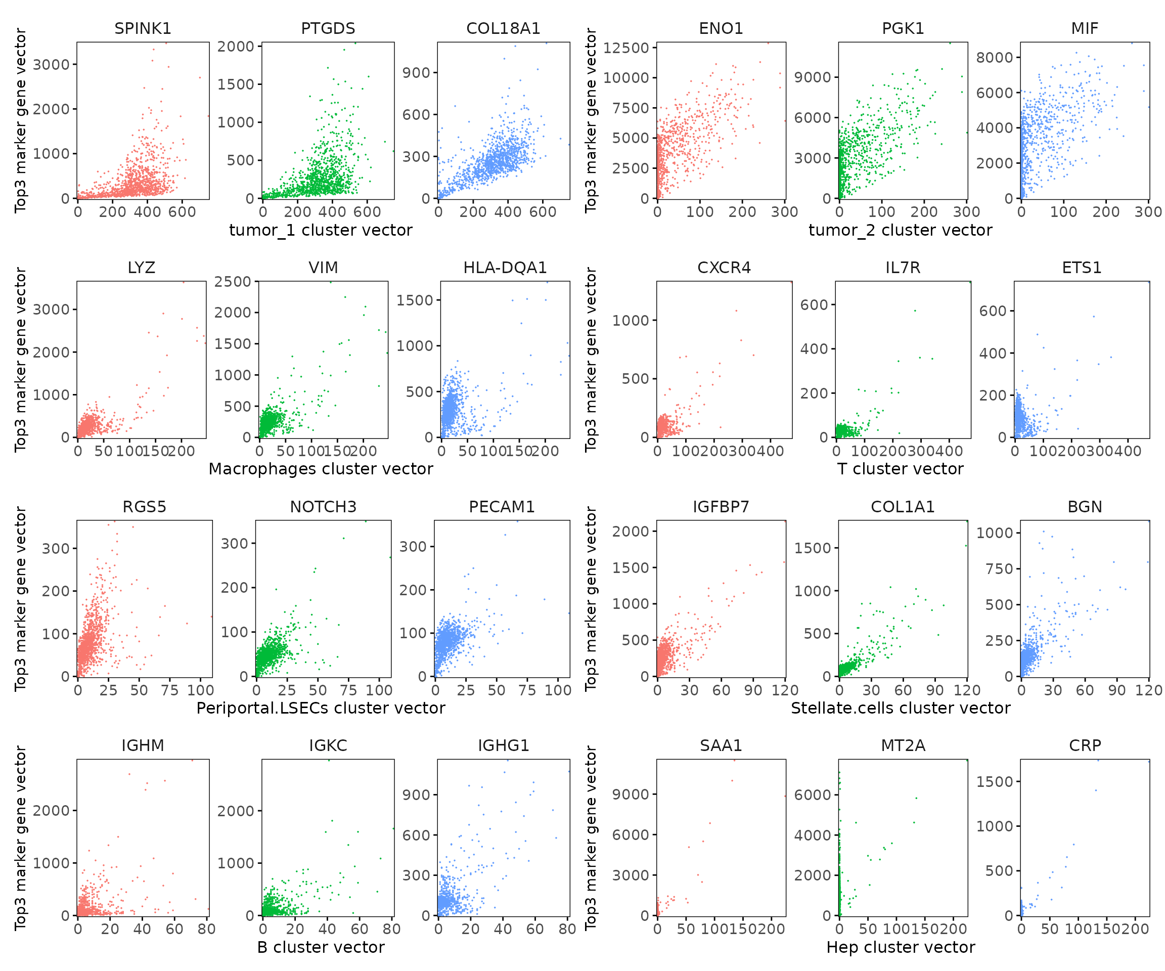
Marker gene summary per cluster
For each cluster, we summarized the detected marker genes and their corresponding strengths. We list genes with model coefficients above the defined cutoff (e.g. 0.1) for each cluster.
Tumor clusters show strong enrichment for proliferative and metabolic genes such as ENO1, PGK1, LDHA, and NDRG1, as well as hypoxia- and stress-related genes (VEGFA, HILPDA, MIF, CRYAB). These are hallmark features of malignant hepatocytes and hypoxic tumor microenvironments. SPINK1 and PTGDS, detected in tumor_1, are known liver cancer–associated genes linked to tumor progression and inflammation.
Macrophages express canonical myeloid and phagocytic markers including LYZ, C1QA/B/C, CD163, and FCGR3A, confirming accurate annotation. Their expression of VIM, ANXA1, and GPNMB suggests activation and tissue-remodeling phenotypes typical of tumor-associated macrophages.
T cells show clear expression of CD3E, IL7R, CXCR4, and ETS1, indicating both cytotoxic and helper T-cell populations.
Stellate cells are characterized by strong collagen and extracellular matrix genes (COL1A1, COL1A2, ACTA2, TAGLN, BGN, MGP), consistent with their myofibroblastic role in the tumor stroma.
Periportal LSECs express PECAM1, KLF2, and RGS5, marking vascular endothelium, while B cells are dominated by immunoglobulin genes (IGHM, IGKC, IGHG1, JCHAIN), reflecting antibody-producing plasma cells.
Hepatocytes display classic liver-enriched genes including SAA1, CRP, MT1X, MT2A, and ARG1, confirming the presence of residual functional hepatic tissue.
## linear modelling
output_data <- do.call(rbind, lapply(cluster_names, function(cl) {
  subset <- jazzPanda_res[jazzPanda_res$top_cluster == cl, ]
  sorted_subset <- subset[order(-subset$glm_coef), ]
  if (length(sorted_subset) == 0){
    return(data.frame(Cluster = cl, Genes = "  "))
  }
  if (cl != "NoSig"){
    gene_list <- paste(sorted_subset$gene, "(", round(sorted_subset$glm_coef, 2), ")", sep="", collapse=", ")
  }else{
    gene_list <- paste(sorted_subset$gene, "", sep="", collapse=", ")
  }

  return(data.frame(Cluster = cl, Genes = gene_list))
}))

knitr::kable(
  output_data,
  caption = "Detected marker genes for each cluster by linear modelling approach in jazzPanda, in decreasing value of glm coefficients"
)| Cluster | Genes |
|---|---|
| tumor_1 | SPINK1(1.14), PTGDS(0.99), COL18A1(0.46), NOTCH1(0.18), IL1RAP(0.16) |
| tumor_2 | ENO1(29.36), PGK1(23.43), MIF(19.02), NDRG1(16.43), VEGFA(13.31), SPP1(9.22), SOX4(6.18), NDUFA4L2(4.79), CRYAB(4.48), JUN(4.08), TPI1(3.75), LDHA(3.67), SERPINA3(3.58), EFNA1(3.56), IGFBP5(3.39), IGFBP3(2.95), POU5F1(2.58), LGALS1(2.48), SOX9(2.43), HSPA1A(2.36), YBX3(2.28), DUSP1(2.19), ZFP36(1.66), CD44(1.57), LGALS3(1.55), SLC2A1(1.22), CD68(1.13), GSN(1.1), VEGFB(1.09), TNFRSF14(1.03), COL9A2(0.98), ITGA5(0.94), GADD45B(0.87), TNXB(0.63), VWA1(0.56), HILPDA(0.54), OSMR(0.36), CELSR1(0.33), SPARCL1(0.3), FOS(0.29), MB(0.26), TGFB1(0.21), WNT9A(0.2), TLR5(0.18), INHBA(0.17), ITGA3(0.16), GAS6(0.13) |
| Macrophages | LYZ(8.43), VIM(4.59), HLA-DQA1(3.87), C1QB(3.64), C1QC(3.39), C1QA(2.39), RGS1(2.08), JUNB(1.99), COTL1(1.99), S100A4(1.82), IFITM1(1.63), MS4A6A(1.35), ANXA1(1.3), GPNMB(1.11), FCGR3A(1.1), ITGB2(1.09), TYROBP(1.07), CD163(1.05), MSR1(0.92), COL6A2(0.92), CRIP1(0.82), CSF1R(0.77), MMP7(0.73), AIF1(0.71), FCER1G(0.65), CD4(0.62), CD53(0.59), ITGAX(0.58), BASP1(0.5), MS4A4A(0.36), ICAM1(0.33), OLR1(0.17), IDO1(0.12) |
| T | CXCR4(1.89), IL7R(1.18), ETS1(1.03), SPOCK2(0.72), CD69(0.55), CXCL13(0.48), IKZF3(0.34), SELL(0.27), CD3E(0.25) |
| Periportal.LSECs | RGS5(2.68), NOTCH3(1.27), PECAM1(1.1), KLF2(0.6) |
| Stellate.cells | IGFBP7(8.93), COL1A1(8), BGN(6.44), ACTA2(4.87), TAGLN(4.62), MGP(3.71), COL4A1(2.95), COL1A2(2.53), C11orf96(2.08), COL4A2(1.92), THBS1(1.85), THBS2(1.8), DCN(1.46), COL5A1(0.91), VCAN(0.23) |
| B | IGHM(22.52), IGKC(13.03), IGHG1(11.27), IGHG2(5.56), IGHA1(5.38), JCHAIN(3.87) |
| Central.venous.LSECs | () |
| Cholangiocytes | () |
| Hep | SAA1(55.18), MT2A(28.62), CRP(8.61), MT1X(4.31), AZGP1(3.26), CD14(1.8), INSIG1(1.69), CXCL12(1.56), IGF2(0.8), ARG1(0.44) |
| Portal.endothelial.cells | () |
| NK.like.cells | () |
| Erthyroid.cells | () |
Correlation approach
We next applied the correlation-based method using the same 40 × 40 binning strategy. This approach highlights genes whose spatial patterns are highly correlated with specific cell type domains.
perm_p = compute_permp(x= list("cancer" = hl_cancer),
                       cluster_info=cluster_info,
                       perm.size=5000,
                       bin_type="square",
                       bin_param=c(grid_length,grid_length),
                       test_genes= all_genes,
                       correlation_method = "pearson",
                       n_cores = 5,
                       correction_method="BH")

saveRDS(perm_p, here(gdata,paste0(data_nm, "_perm_lst.Rds")))
We can get the correlation between every gene and cluster using the
get_cor function, which quantifies how strongly each gene’s
spatial expression pattern aligns with the spatial distribution of each
cluster.
To assess statistical significance, permutation testing results are
retrieved from the saved perm_lst object. The corresponding raw p-values
can be obtained with get_perm_p, and the
multiple-testing–adjusted p-values with get_perm_adjp.
These adjusted p-values help identify genes that are significantly
associated with specific spatial domains after controlling for random
spatial correlations.
# load from saved objects
perm_lst = readRDS(here(gdata,paste0(data_nm, "_perm_lst.Rds")))
perm_res = get_perm_adjp(perm_lst)
obs_corr = get_cor(perm_lst)
For every cluster, genes were selected if they passed permutation significance and exceeded the 75th percentile of observed correlation values, with the top 10 highest correlations retained for visualization.
The top markers identified by the jazzPanda correlation method capture spatially enriched genes whose expression patterns correlate strongly with local cell-type density. The dot plot below summarizes the top 10 genes per cluster, with dot size representing detection frequency and color reflecting mean expression.
top_mg_corr <- data.frame(cluster = character(),
                          gene    = character(),
                          corr    = numeric(),
                          stringsAsFactors = FALSE)
for (cl in cluster_names) {
  obs_cutoff <- quantile(obs_corr[, cl], 0.75, na.rm = TRUE)
  perm_cl <- intersect(
    rownames(perm_res[perm_res[, cl] < 0.05, ]),
    rownames(obs_corr[obs_corr[, cl] > obs_cutoff, ])
  )
  if (length(perm_cl) > 0) {
    selected_rows <- obs_corr[perm_cl, , drop = FALSE]
    ord <- order(selected_rows[, cl], decreasing = TRUE,
                 na.last = NA)
    top_genes <- head(rownames(selected_rows)[ord], 5)
    top_vals  <- head(selected_rows[ord, cl], 5)

    top_mg_corr <- rbind(
      top_mg_corr,
      data.frame(cluster = rep(cl, length(top_genes)),
                 gene    = top_genes,
                 corr    = top_vals,
                 stringsAsFactors = FALSE)
    )
  }
}


p1<-DotPlot(seu, features = unique(top_mg_corr$gene)) +
     scale_colour_gradient(low = "white", high = "red") +
    coord_flip()+
    theme(axis.text.x = element_text(angle = 45, hjust = 1, vjust = 1))+
    labs(title = "Top 10 marker genes (jazzPanda-correlation)",
         x="", y="")

p1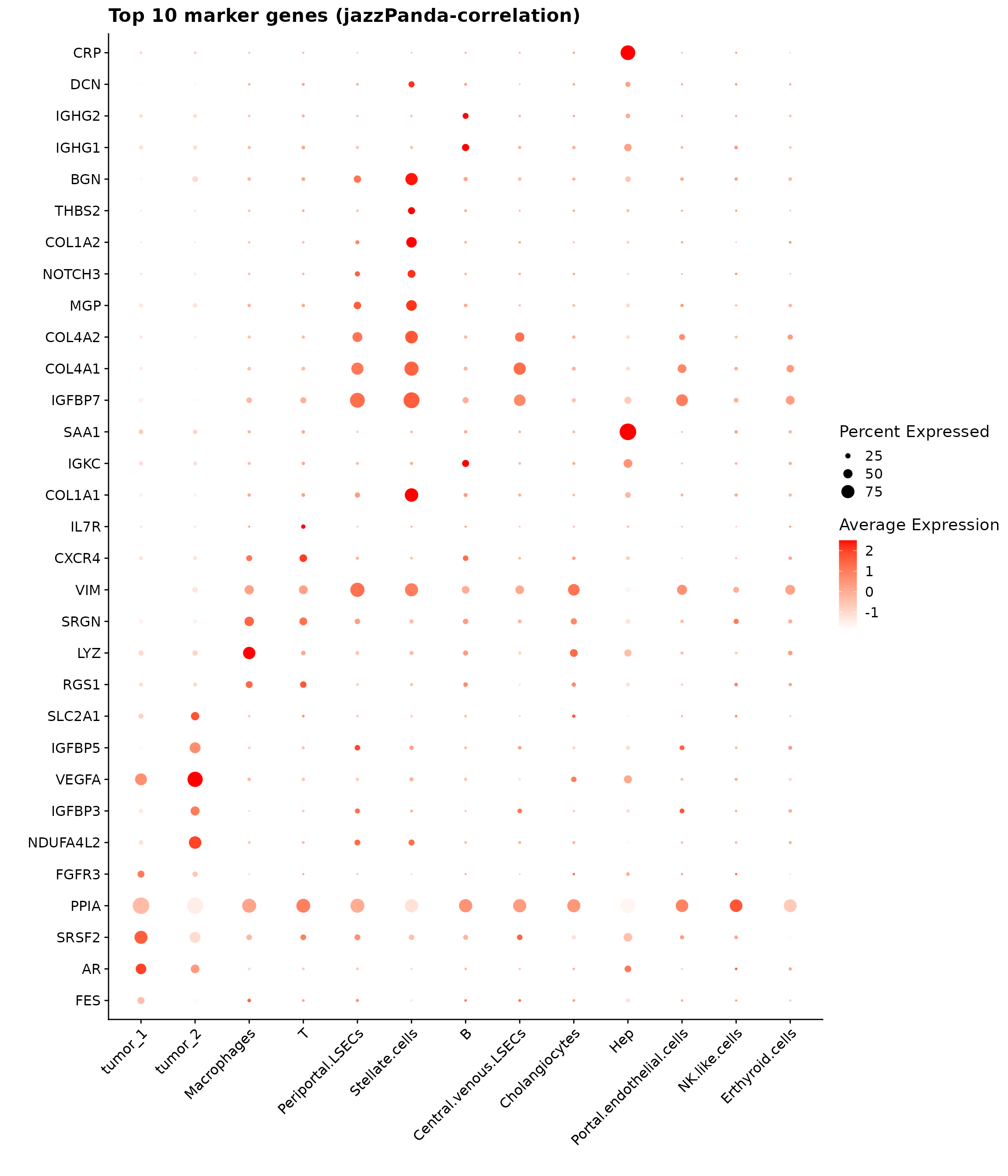
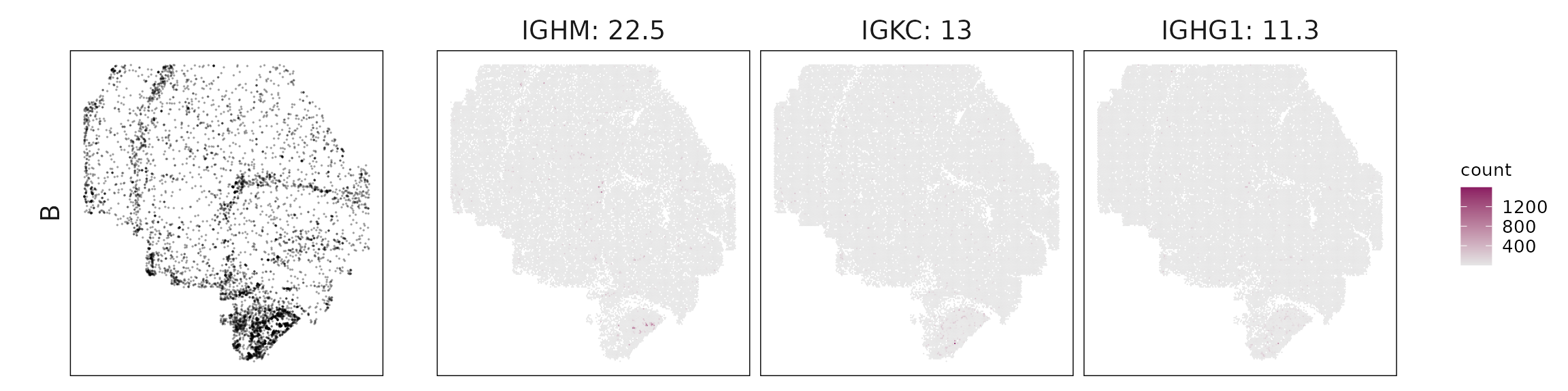
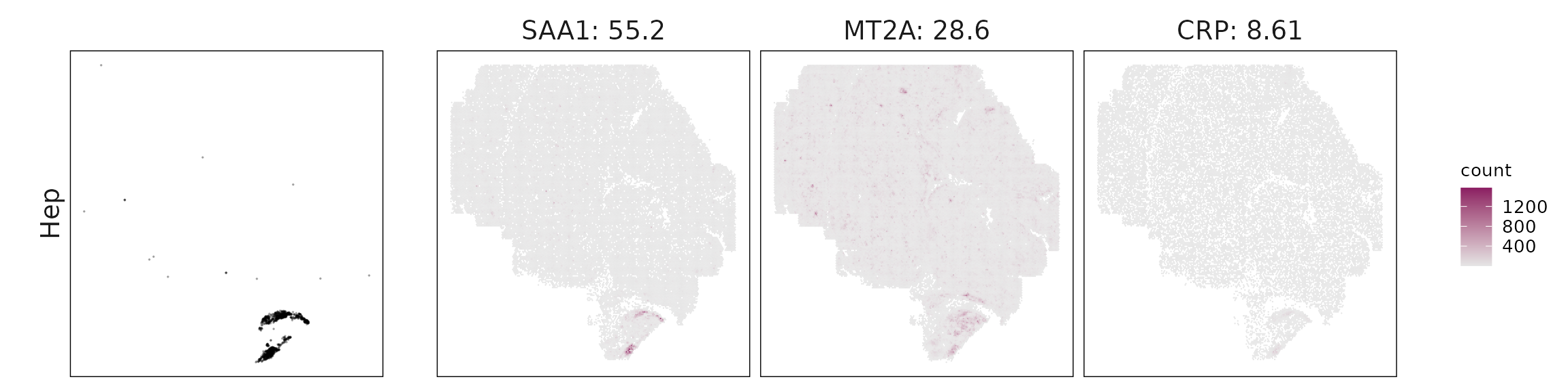
Top3 marker genes by jazzPanda_correlation
For each cluster, the top three genes with the highest significant correlations were visualized alongside the spatial cluster map. The spatial patterns of these marker genes closely align with the distribution of their associated clusters, confirming that the correlation approach captures coherent spatial co-localization between genes and cell-type domains.
for (cl in cluster_names){
    obs_cutoff = quantile(obs_corr[, cl], 0.75)
    perm_cl<-intersect(row.names(perm_res[perm_res[,cl]<0.05,]),
                     row.names(obs_corr[obs_corr[, cl]>obs_cutoff,]))
    inters<-perm_cl
    rounded_val<-signif(as.numeric(obs_corr[inters,cl]), digits = 3)
    inters_df = as.data.frame(cbind(gene=inters, value=rounded_val))
    inters_df$value = as.numeric(inters_df$value)
    inters_df<-inters_df[order(inters_df$value, decreasing = TRUE),]
    inters_df$text= paste(inters_df$gene,inters_df$value,sep=": ")

    if (length(inters > 0)){
        inters_df = inters_df[1:min(3, nrow(inters_df)),]
        inters = inters_df$gene
        iters_sp1= hl_cancer$feature_name %in% inters
        vis_r1 =hl_cancer[iters_sp1,
                        c("x","y","feature_name")]
        vis_r1$value = inters_df[match(vis_r1$feature_name,inters_df$gene),
                        "value"]
        vis_r1=vis_r1[order(vis_r1$value,decreasing = TRUE),]
        vis_r1$text_label= paste(vis_r1$feature_name,
                            vis_r1$value,sep=": ")
        vis_r1$text_label=factor(vis_r1$text_label, levels=inters_df$text)

        vis_r1 = vis_r1[order(vis_r1$text_label),]

        genes_plt <- plot_top3_genes(vis_df=vis_r1, fig_ratio=fig_ratio)

        cluster_data =  cluster_info[cluster_info$cluster==cl, ]
        cl_pt<- ggplot(data =cluster_data,
                    aes(x = x, y = y, color=sample))+
                    #geom_hex(bins = 100)+
                    geom_point(size=0.001, alpha=0.3)+
                    facet_wrap(~anno_name, nrow=1,strip.position = "left")+
                    scale_color_manual(values = c("black"))+
                    defined_theme +
            theme(legend.position = "none",
                    strip.background = element_blank(),
                    legend.key.width = unit(15, "cm"),
                    aspect.ratio = fig_ratio,
                    plot.margin = margin(0, 0, 0, 0),
                    strip.text = element_text(size = rel(1.3)))

        layout_design <- (wrap_plots(cl_pt, ncol = 1) | genes_plt) +
            plot_layout(widths = c(1, 3), heights = c(1))

        print(layout_design)
    }
  }
Cluster vector versus marker gene vector
We further examined the quantitative relationship between the cluster vector and its top correlated marker gene vectors. Each scatter plot compares the spatial strength of a marker gene with the corresponding cluster vector across spatial bins. The results show clear positive linear relationships, indicating that the marker genes are spatially aligned with the inferred cluster domain.
plot_lst=list()
for (cl in cluster_names){
    obs_cutoff = quantile(obs_corr[, cl], 0.75)
    perm_cl<-intersect(row.names(perm_res[perm_res[,cl]<0.05,]),
                     row.names(obs_corr[obs_corr[, cl]>obs_cutoff,]))
    inters<-perm_cl
    if (length(inters) >0){
        rounded_val<-signif(as.numeric(obs_corr[inters,cl]), digits = 3)
        inters_df = as.data.frame(cbind(gene=inters, value=rounded_val))
        inters_df$value = as.numeric(inters_df$value)
        inters_df<-inters_df[order(inters_df$value, decreasing = TRUE),]

        inters_df = inters_df[1:min(3, nrow(inters_df)),]
        mk_genes = inters_df$gene

        dff = as.data.frame(cbind(sv_lst$cluster_mt[,cl],
                          sv_lst$gene_mt[,mk_genes]))
        colnames(dff) = c("cluster", mk_genes)
        dff$vector_id = c(1:nbins)
        long_df <- dff %>%
         tidyr::pivot_longer(cols = -c(cluster, vector_id), names_to = "gene",
           values_to = "vector_count")
        long_df$gene = factor(long_df$gene, levels=mk_genes)
        p<-ggplot(long_df, aes(x = cluster, y = vector_count, color=gene )) +
        geom_point(size=0.01) +
        facet_wrap(~gene, scales="free_y", nrow=1) +
        labs(x = paste(cl, " cluster vector ", sep=""),
        y = "Top3 marker gene vector") +
        theme_minimal()+
        scale_y_continuous(expand = c(0.01,0.01))+
        scale_x_continuous(expand =  c(0.01,0.01))+
        theme(panel.grid = element_blank(),
          legend.position = "none",
        strip.text = element_text(size = 12),
        axis.line=element_blank(),
        axis.text=element_text(size = 11),
        axis.ticks=element_line(color="black"),
        axis.title.y=element_text(size = 11),
         axis.title.x=element_text(size = 12),
        panel.border  =element_rect(colour = "black",
                                fill=NA, linewidth=0.5)
        )

        if (length(mk_genes) == 2) {
            p <- (p | plot_spacer()) +
            plot_layout(widths = c(2, 1))
        } else if (length(mk_genes) == 1) {
            p <- (p | plot_spacer() | plot_spacer()) +
            plot_layout(widths = c(1, 1, 1))
        }

        plot_lst[[cl]] = p
    }
}


combined_plot <- wrap_plots(plot_lst, ncol = 2)

combined_plot 
Marker gene summary per cluster
The correlation method identified spatially co-expressed genes aligned with cell-type distributions, though some overlap between adjacent compartments is evident.
Tumor 1: Broad set of highly correlated oncogenic and metabolic genes (STAT3, EGFR, MTOR, HIF1A, CD274), reflecting general tumor activity but also over-selection of housekeeping genes.
Tumor 2: Coherent hypoxia and glycolysis signature (NDUFA4L2, IGFBP3, VEGFA, ENO1, PGK1, SPP1), consistent with metabolically active tumor regions.
Macrophages: Strong immune–stromal markers (LYZ, RGS1, SRGN, VIM, ANXA1), typical of TAMs; partial mixing with B-cell zones suggested by immunoglobulin hits.
T cells: IL7R and CXCR4 confirm activated tissue-resident T cells, while COL1A1 and SAA1 reflect spatial overlap with stromal/hepatic areas.
Periportal LSECs: Vascular and ECM genes (IGFBP7, COL4A1/2, MGP, NOTCH3, ACTA2) mark endothelial identity with expected stromal proximity.
Stellate cells: Classic fibroblast signature (COL1A1/2, THBS2, BGN, DCN, ACTA2), accurately capturing activated stellate programs.
B cells: Dominated by immunoglobulin genes (IGHG1/2, IGKC, IGHM, JCHAIN), confirming B-lineage identity.
Hepatocytes: Liver-specific acute-phase genes (CRP, SAA1) validate annotation; minor stromal signals due to small spatial domain.
Other clusters: No distinct markers detected, likely reflecting low abundance or diffuse signal.
It is important to inspect and adjust this cutoff as needed — in some cases, the 75th percentile threshold may still fall below 0.1, which could include weakly correlated genes. A higher cutoff can be applied to ensure that only strongly spatially associated genes are retained.
# correlation appraoch
# Combine into a new dataframe for LaTeX output
output_data <- do.call(rbind, lapply(cluster_names, function(cl) {
  obs_cutoff = quantile(obs_corr[, cl], 0.75)
  perm_cl=intersect(row.names(perm_res[perm_res[,cl]<0.05,]),
                   row.names(obs_corr[obs_corr[, cl]>obs_cutoff,]))

  if (length(perm_cl) == 0){
    return(data.frame(Cluster = cl, Genes = "  "))
  }
  sorted_subset = obs_corr[row.names(obs_corr) %in% perm_cl,]
  sorted_subset <- sorted_subset[order(-sorted_subset[,cl]), ]
  if (cl != "NoSig"){
    gene_list <- paste(row.names(sorted_subset), "(", round(sorted_subset[,cl], 2), ")", sep="", collapse=", ")
  }else{
    gene_list <- paste(row.names(sorted_subset), "", sep="", collapse=", ")
  }

  return(data.frame(Cluster = cl, Genes = gene_list))
}))
knitr::kable(
  output_data,
  caption = "Detected marker genes for each cluster by correlation approach in jazzPanda, in decreasing value of observed correlation"
)| Cluster | Genes |
|---|---|
| tumor_1 | FES(0.94), AR(0.94), SRSF2(0.94), PPIA(0.94), FGFR3(0.93), ZBTB16(0.93), XBP1(0.93), NR1H3(0.93), TNFRSF11B(0.93), THSD4(0.93), IRF3(0.93), IGF1(0.93), ARF1(0.93), HDAC1(0.93), RARA(0.93), MTOR(0.93), HDAC4(0.93), DUSP6(0.92), RXRB(0.92), ACACB(0.92), NR2F2(0.92), RPL21(0.92), ATR(0.92), XCL1(0.92), TYK2(0.92), DNMT1(0.92), STAT3(0.92), ATP5F1E(0.92), EZH2(0.92), CDH1(0.92), PCNA(0.92), VHL(0.92), EIF5A(0.92), BTF3(0.92), NOSIP(0.92), NR1H2(0.92), RPL37(0.92), SMAD2(0.92), SNAI1(0.92), AQP3(0.92), CCL15(0.92), ACVR1B(0.92), NOTCH1(0.92), FKBP5(0.92), ABL1(0.92), TUBB(0.92), IL6R(0.92), IL15RA(0.92), HMGN2(0.92), GLUD1(0.92), NFKB1(0.92), HDAC3(0.92), DNMT3A(0.92), HSP90B1(0.92), IL11RA(0.91), COL9A3(0.91), BAX(0.91), FAU(0.91), PDS5A(0.91), NFKBIA(0.91), UBA52(0.91), APOE(0.91), PTK2(0.91), SNAI2(0.91), EGFR(0.91), ATP5F1B(0.91), FASN(0.91), PROX1(0.91), BRAF(0.91), CTNNB1(0.91), RNF43(0.91), BID(0.91), SMARCB1(0.91), RPL34(0.91), WNT3(0.91), RXRA(0.91), MAPK13(0.91), MALAT1(0.91), IL1RAP(0.91), IL1RN(0.91), CDKN1A(0.91), IL13RA1(0.91), HSPB1(0.91), SMAD4(0.91), BECN1(0.91), IL17RA(0.91), SEC23A(0.91), FKBP11(0.91), LGALS3BP(0.91), PFN1(0.91), HLA-A(0.91), TAP2(0.91), ICA1(0.91), NEAT1(0.91), MMP1(0.91), PSD3(0.91), SLCO2B1(0.91), ERBB3(0.91), ADIRF(0.91), TNNC1(0.91), GSTP1(0.91), HSP90AA1(0.91), KRAS(0.91), BTG1(0.91), ATG5(0.91), KRT15(0.91), TYMS(0.91), EFNA5(0.91), SEC61G(0.91), RACK1(0.91), ITGAM(0.91), STAT5B(0.91), CHEK2(0.91), RPL22(0.9), CAMP(0.9), KRT86(0.9), MYL12A(0.9), CSK(0.9), RARRES2(0.9), INHA(0.9), PTGES3(0.9), CASP3(0.9), SMO(0.9), INHBB(0.9), FZD6(0.9), LTBR(0.9), ATM(0.9), CD63(0.9), PLD3(0.9), MAP1LC3B(0.9), BCL2L1(0.9), SERPINH1(0.9), MAPK14(0.9), ACVR1(0.9), ATG12(0.9), AKT1(0.9), FZD5(0.9), INSR(0.9), RORA(0.9), ATG10(0.9), PLCG1(0.9), ABL2(0.9), HMGB2(0.9), VCAM1(0.9), CELSR2(0.9), RPL32(0.9), ACE(0.9), YES1(0.9), MZT2A(0.9), STAT6(0.9), CHEK1(0.9), SLC40A1(0.9), ERBB2(0.9), H4C3(0.9), BST2(0.9), BMPR2(0.9), CD274(0.9), NACA(0.9), HSP90AB1(0.9), ST6GAL1(0.9), CSTB(0.9), KDR(0.9), CXCL16(0.9), PARP1(0.9), DST(0.9), ACVR2A(0.9), FGFR2(0.9), RYK(0.9), DHRS2(0.9), IFNGR2(0.9), IL10RB(0.9), CSF1(0.9), IFNAR1(0.9), APOC1(0.9), SH3BGRL3(0.9), TUBB4B(0.9), PPARA(0.9), SELENOP(0.9), PTGES2(0.89), PDGFC(0.89), ITM2B(0.89), TNFRSF1A(0.89), B2M(0.89), ADGRG1(0.89), GLUL(0.89), IL1A(0.89), CD276(0.89), SOD1(0.89), CDKN3(0.89), EPHB4(0.89), TPM2(0.89), LEP(0.89), CFLAR(0.89), PHLDA2(0.89), ADGRA3(0.89), CAV1(0.89), TOX(0.89), CYSTM1(0.89), MST1R(0.89), CX3CL1(0.89), GSK3B(0.89), CD9(0.89), HIF1A(0.89), IFNAR2(0.89), CALM1(0.89), HMGCS1(0.89), NR3C1(0.89), BMPR1A(0.89), NUSAP1(0.89), EGF(0.89), CCL17(0.89), CD81(0.89), H2AZ1(0.89), RAC1(0.89), HSD17B2(0.89), RELA(0.89) |
| tumor_2 | NDUFA4L2(0.81), IGFBP3(0.79), VEGFA(0.77), IGFBP5(0.76), SLC2A1(0.71), ENO1(0.7), PGK1(0.69), SPP1(0.63) |
| Macrophages | RGS1(0.82), LYZ(0.8), SRGN(0.8), VIM(0.79), CXCR4(0.78), COL1A1(0.76), ANXA1(0.75), TAGLN(0.7), BGN(0.69), IL7R(0.67), DCN(0.67), COL1A2(0.66), IGHG1(0.63), IGKC(0.53), IGHM(0.46), SAA1(0.38) |
| T | IL7R(0.77), CXCR4(0.74), COL1A1(0.64), IGKC(0.53), SAA1(0.45), CRP(0.42) |
| Periportal.LSECs | IGFBP7(0.81), COL4A1(0.79), COL4A2(0.79), MGP(0.79), NOTCH3(0.75), ACTA2(0.74), VIM(0.74), TAGLN(0.7), BGN(0.7), COL1A2(0.7), COL1A1(0.66) |
| Stellate.cells | COL1A1(0.88), COL1A2(0.84), THBS2(0.78), IGFBP7(0.75), BGN(0.75), DCN(0.73), TAGLN(0.69), ACTA2(0.65), IGKC(0.59), SAA1(0.36) |
| B | IGHG1(0.71), COL1A1(0.66), IGKC(0.65), IGHG2(0.62), DCN(0.61), IL7R(0.58), COL1A2(0.55), IGHM(0.52), IGHA1(0.5), JCHAIN(0.47), SAA1(0.44), CRP(0.4) |
| Central.venous.LSECs | |
| Cholangiocytes | |
| Hep | CRP(0.91), SAA1(0.9), DCN(0.54), IGKC(0.53), IL7R(0.44), IGHG1(0.42) |
| Portal.endothelial.cells | |
| NK.like.cells | |
| Erthyroid.cells |
limma
We applied the limma framework to identify differentially expressed marker genes across clusters in the liver cancer sample. Count data were normalized using log-transformed counts from the speckle package. A linear model was fitted for each gene with cluster identity as the design factor, and pairwise contrasts were constructed to compare each cluster against all others. Empirical Bayes moderation was applied to stabilize variance estimates, and significant genes were determined using the moderated t-statistics from eBayes.
y <- DGEList(counts_cancer_sample[, cluster_info$cell_id])
y$genes <-row.names(counts_cancer_sample)

logcounts <- speckle::normCounts(y,log=TRUE,prior.count=0.1)
maxclust <- length(unique(cluster_info$cluster))

grp <- cluster_info$cluster

design <- model.matrix(~0+grp)
colnames(design) <- levels(grp)

mycont <- matrix(NA,ncol=length(levels(grp)),nrow=length(levels(grp)))
rownames(mycont)<-colnames(mycont)<-levels(grp)
diag(mycont)<-1
mycont[upper.tri(mycont)]<- -1/(length(levels(factor(grp)))-1)
mycont[lower.tri(mycont)]<- -1/(length(levels(factor(grp)))-1)
fit <- lmFit(logcounts,design)
fit.cont <- contrasts.fit(fit,contrasts=mycont)
fit.cont <- eBayes(fit.cont,trend=TRUE,robust=TRUE)

limma_dt<-decideTests(fit.cont)

summary(limma_dt)

saveRDS(fit.cont, here(gdata,paste0(data_nm, "_fit_cont_obj.Rds")))
fit.cont = readRDS(here(gdata,paste0(data_nm, "_fit_cont_obj.Rds")))
limma_dt <- decideTests(fit.cont)
summary(limma_dt) tumor_1 tumor_2 Macrophages T Periportal.LSECs Stellate.cells B
Down 268 205 654 450 647 746 502
NotSig 134 128 147 255 143 106 352
Up 598 667 199 295 210 148 146
Central.venous.LSECs Cholangiocytes Hep Portal.endothelial.cells
Down 529 435 212 638
NotSig 346 440 447 303
Up 125 125 341 59
NK.like.cells Erthyroid.cells
Down 414 69
NotSig 475 915
Up 111 16top_markers <- lapply(cluster_names, function(cl) {
tt <- topTable(fit.cont,
coef = cl,
number = Inf,
adjust.method = "BH",
sort.by = "P")
tt <- tt[order(tt$adj.P.Val, -abs(tt$logFC)), ]
tt$contrast <- cl
tt$gene <- rownames(tt)
head(tt, 10)
})
# Combine into one data.frame
top_markers_df <- bind_rows(top_markers) %>%
select(contrast, gene, logFC, adj.P.Val)
p1<- DotPlot(seu, features = unique(top_markers_df$gene)) +
scale_colour_gradient(low = "white", high = "red") +
coord_flip()+
theme(axis.text.x = element_text(angle = 45, hjust = 1, vjust = 1))+
labs(title = "Top 10 marker genes (limma)", x="", y="")
p1
Wilcoxon Rank Sum Test
The FindAllMarkers function applies a Wilcoxon Rank Sum
test to detect genes with cluster-specific expression shifts. Only
positive markers (upregulated genes) were retained using a log
fold-change threshold of 0.1.
hlc_seu=CreateSeuratObject(counts = counts_cancer_sample[, cluster_info$cell_id], project = "hl_cancer")
Idents(hlc_seu) = cluster_info[match(colnames(hlc_seu),
                                      cluster_info$cell_id),"cluster"]
hlc_seu = NormalizeData(hlc_seu, verbose = FALSE,
                        normalization.method = "LogNormalize")
hlc_seu = FindVariableFeatures(hlc_seu, selection.method = "vst",
                               nfeatures = 1000, verbose = FALSE)

hlc_seu=ScaleData(hlc_seu, verbose = FALSE)

set.seed(989)
# print(ElbowPlot(hlc_seu, ndims = 50))
hlc_seu <- RunPCA(hlc_seu, features = row.names(hlc_seu),
                  npcs = 30, verbose = FALSE)
hlc_seu <- RunUMAP(object = hlc_seu, dims = 1:15)


seu_markers <- FindAllMarkers(hlc_seu, only.pos = TRUE,logfc.threshold = 0.1)


saveRDS(seu_markers, here(gdata,paste0(data_nm, "_seu_markers.Rds")))

saveRDS(hlc_seu, here(gdata,paste0(data_nm, "_seu.Rds")))
FM_result= readRDS(here(gdata,paste0(data_nm, "_seu_markers.Rds")))
FM_result = FM_result[FM_result$avg_log2FC>0.1, ]
table(FM_result$cluster)
                 tumor_1                  tumor_2              Macrophages
                     131                      130                      756
                       T         Periportal.LSECs           Stellate.cells
                     804                      744                      694
                       B     Central.venous.LSECs           Cholangiocytes
                     768                      746                      740
                     Hep Portal.endothelial.cells            NK.like.cells
                     161                      726                      656
         Erthyroid.cells
                     138
FM_result$cluster <- factor(FM_result$cluster,
levels = cluster_names)
top_mg <- FM_result %>%
group_by(cluster) %>%
arrange(desc(avg_log2FC), .by_group = TRUE) %>%
slice_max(order_by = avg_log2FC, n = 10) %>%
select(cluster, gene, avg_log2FC)
p1<-DotPlot(seu, features = unique(top_mg$gene)) +
scale_colour_gradient(low = "white", high = "red") +
coord_flip()+
theme(axis.text.x = element_text(angle = 45, hjust = 1, vjust = 1))+
labs(title = "Top 10 marker genes (WRS)", x="", y="")
p1
# Combine into a new dataframe for LaTeX output
# output_data <- do.call(rbind, lapply(cluster_names, function(cl) {
# subset <- top_mg[top_mg$cluster == cl, ]
# sorted_subset <- subset[order(-subset$avg_log2FC), ]
# gene_list <- paste(sorted_subset$gene, "(", round(sorted_subset$avg_log2FC, 2), ")", sep="", collapse=", ")
#
# return(data.frame(Cluster = cl, Genes = gene_list))
# }))
# latex_table <- xtable(output_data, caption="Detected marker genes for each cluster by FindMarkers")
# print.xtable(latex_table, include.rownames = FALSE, hline.after = c(-1, 0, nrow(output_data)), comment = FALSE)
Comparison of marker gene detection methods
Cumulative rank plot
We compared the performance of different marker detection methods — jazzPanda (linear modelling and correlation), limma, and Seurat’s Wilcoxon Rank Sum test — by comparing the cumulative average spatial correlation between ranked marker genes and their corresponding target clusters at the spatial vector level.
Across multiple cell populations, including tumor subclusters, periportal LSECs, stellate cells, macrophages, and T cells, jazzPanda consistently prioritized genes with higher spatial concordance. In contrast, Wilcoxon and limma markers rarely achieve high correlation, indicating that classical differential expression approaches identify genes with large expression differences but limited spatial coherence.
plot_lst=list()
cor_M = cor(sv_lst$gene_mt,
            sv_lst$cluster_mt[, cluster_names],
            method = "spearman")

Idents(seu)=cluster_info$cluster[match(colnames(seu),
                                       cluster_info$cell_id)]
for (cl in cluster_names){

    fm_cl=FindMarkers(seu, ident.1 = cl, only.pos = TRUE,
            logfc.threshold = 0.1)
    fm_cl = fm_cl[fm_cl$p_val_adj<0.05, ]
    fm_cl = fm_cl[order(fm_cl$avg_log2FC, decreasing = TRUE),]
    to_plot_fm =row.names(fm_cl)
    if (length(to_plot_fm)>0){
        FM_pt =FM_pt = data.frame("name"=to_plot_fm,"rk"= 1:length(to_plot_fm),
                       "y"= get_cmr_ma(to_plot_fm,cor_M = cor_M, cl = cl),
                       "type"="Wilcoxon Rank Sum Test")
    }else{
        FM_pt <- data.frame(name = character(0), rk = integer(0),
                               y= numeric(0), type = character(0))
    }

    limma_cl<-topTable(fit.cont,coef=cl,p.value = 0.05, n=Inf, sort.by = "p")
    limma_cl = limma_cl[limma_cl$logFC>0, ]
    to_plot_lm = row.names(limma_cl)
    if (length(to_plot_lm)>0){
         limma_pt = data.frame("name"=to_plot_lm,"rk"= 1:length(to_plot_lm),
                                  "y"= get_cmr_ma(to_plot_lm,cor_M = cor_M, cl = cl),
                                  "type"="limma")
    }else{
        limma_pt <- data.frame(name = character(0), rk = integer(0),
                               y= numeric(0), type = character(0))
    }

    obs_cutoff = quantile(obs_corr[, cl], 0.75)
    perm_cl=intersect(row.names(perm_res[perm_res[,cl]<0.05,]),
                 row.names(obs_corr[obs_corr[, cl]>obs_cutoff,]))
    if (length(perm_cl) > 0) {
        rounded_val=signif(as.numeric(obs_corr[perm_cl,cl]), digits = 3)
        roudned_pval=signif(as.numeric(perm_res[perm_cl,cl]), digits = 3)
        perm_sorted = as.data.frame(cbind(gene=perm_cl, value=rounded_val, pval=roudned_pval))
        perm_sorted$value = as.numeric(perm_sorted$value)
        perm_sorted$pval = as.numeric(perm_sorted$pval)
        perm_sorted=perm_sorted[order(-perm_sorted$pval,
                                  perm_sorted$value,
                                  decreasing = TRUE),]
        corr_pt = data.frame("name"=perm_sorted$gene,"rk"= 1:length(perm_sorted$gene),
                     "y"= get_cmr_ma(perm_sorted$gene,cor_M = cor_M, cl = cl),
                     "type"="jazzPanda-correlation")
    } else {
      corr_pt <-data.frame(name = character(0), rk = integer(0),
                               y= numeric(0), type = character(0))
    }

    lasso_sig = jazzPanda_res[jazzPanda_res$top_cluster==cl,]
    if (nrow(lasso_sig) > 0) {
        lasso_sig <- lasso_sig[order(lasso_sig$glm_coef, decreasing = TRUE), ]
        lasso_pt = data.frame("name"=lasso_sig$gene,"rk"= 1:nrow(lasso_sig),
                          "y"= get_cmr_ma(lasso_sig$gene,cor_M = cor_M, cl = cl),
                          "type"="jazzPanda-glm")
    } else {
      lasso_pt <- data.frame(name = character(0), rk = integer(0),
                               y= numeric(0), type = character(0))
    }

    data_lst = rbind(limma_pt, FM_pt,corr_pt,lasso_pt)

    data_lst$type <- factor(data_lst$type,
                            levels = c("jazzPanda-correlation" ,
                                       "jazzPanda-glm",
                                       "limma", "Wilcoxon Rank Sum Test"))
    data_lst$rk = as.numeric(data_lst$rk)
    cl = sub(cl, pattern = ".cells", replacement="")
    p <-ggplot(data_lst, aes(x = rk, y = y, color = type)) +
        geom_step(size = 0.8) +  # type = "s"
        scale_color_manual(values = c("jazzPanda-correlation" = "orange",
                                    "jazzPanda-glm" = "red",
                                    "limma" = "black",
                                    "Wilcoxon Rank Sum Test" = "blue")) +
        scale_x_continuous(limits = c(0, 50))+
        labs(title = paste(cl, "cells"), x = "Rank of marker genes",
             y = "Cumulative average correlation",
             color = NULL) +
        theme_classic(base_size = 12) +
        theme(plot.title = element_text(hjust = 0.5),
            axis.line = element_blank(),
            panel.border = element_rect(color = "black",
                                        fill = NA, linewidth = 1),
            legend.position = "inside",
            legend.position.inside = c(0.98, 0.02),
            legend.justification = c("right", "bottom"),
            legend.background = element_rect(color = "black",
                                             fill = "white", linewidth = 0.5),
            legend.box.background = element_rect(color = "black",
                                                 linewidth = 0.5)
        )
    plot_lst[[cl]] <- p
}


combined_plot <- wrap_plots(plot_lst, ncol =3)

combined_plot 
Upset plot
We further visualized the overlap between marker genes detected by the four methods using UpSet plots for each cluster.
The limited overlap between jazzPanda and classical tests highlights that spatial modelling captures complementary signal beyond differential expression alone. In particular, the linear modelling approach identifies spatially structured genes that are not necessarily the most differentially expressed but show strong spatial association with cell-type domains. Conversely, Wilcoxon and limma yield smaller, largely overlapping sets dominated by high-abundance genes lacking spatial specificity.
plot_lst=list()
for (cl in cluster_names){
    findM_sig <- FM_result[FM_result$cluster==cl & FM_result$p_val_adj<0.05,"gene"]
    limma_sig <- row.names(limma_dt[limma_dt[,cl]==1,])
    lasso_cl <- jazzPanda_res[jazzPanda_res$top_cluster==cl, "gene"]

    obs_cutoff = quantile(obs_corr[, cl], 0.75)
    perm_cl=intersect(row.names(perm_res[perm_res[,cl]<0.05,]),
                 row.names(obs_corr[obs_corr[, cl]>obs_cutoff,]))

    df_mt <- as.data.frame(matrix(FALSE,nrow=nrow(jazzPanda_res),ncol=4))
    row.names(df_mt) <- jazzPanda_res$gene
    colnames(df_mt) <- c("jazzPanda-glm",
                      "jazzPanda-correlation",
                      "Wilcoxon Rank Sum Test","limma")
    df_mt[findM_sig,"Wilcoxon Rank Sum Test"] <- TRUE
    df_mt[limma_sig,"limma"] <- TRUE
    df_mt[lasso_cl,"jazzPanda-glm"] <- TRUE
    df_mt[perm_cl,"jazzPanda-correlation"] <- TRUE

    df_mt$gene_name <- row.names(df_mt)
    p = upset(df_mt,
               intersect=c("Wilcoxon Rank Sum Test", "limma",
                           "jazzPanda-correlation","jazzPanda-glm"),
               wrap=TRUE, keep_empty_groups= FALSE, name="",
               stripes='white',
               sort_intersections_by ="cardinality",
               sort_sets= FALSE,min_degree=1,
               set_sizes =(
                   upset_set_size()
                   + theme(axis.title= element_blank(),
                           axis.ticks.y = element_blank(),
                           axis.text.y = element_blank())),
               sort_intersections= "descending", warn_when_converting=FALSE,
               warn_when_dropping_groups=TRUE,encode_sets=TRUE,
               width_ratio=0.3, height_ratio=1/4)+
             ggtitle(paste(cl,"cells"))+
                 ggtitle(cl)+
                 theme(plot.title = element_text( size=15))


    plot_lst[[cl]] <- p
}

combined_plot <- wrap_plots(plot_lst, ncol =3)

combined_plot 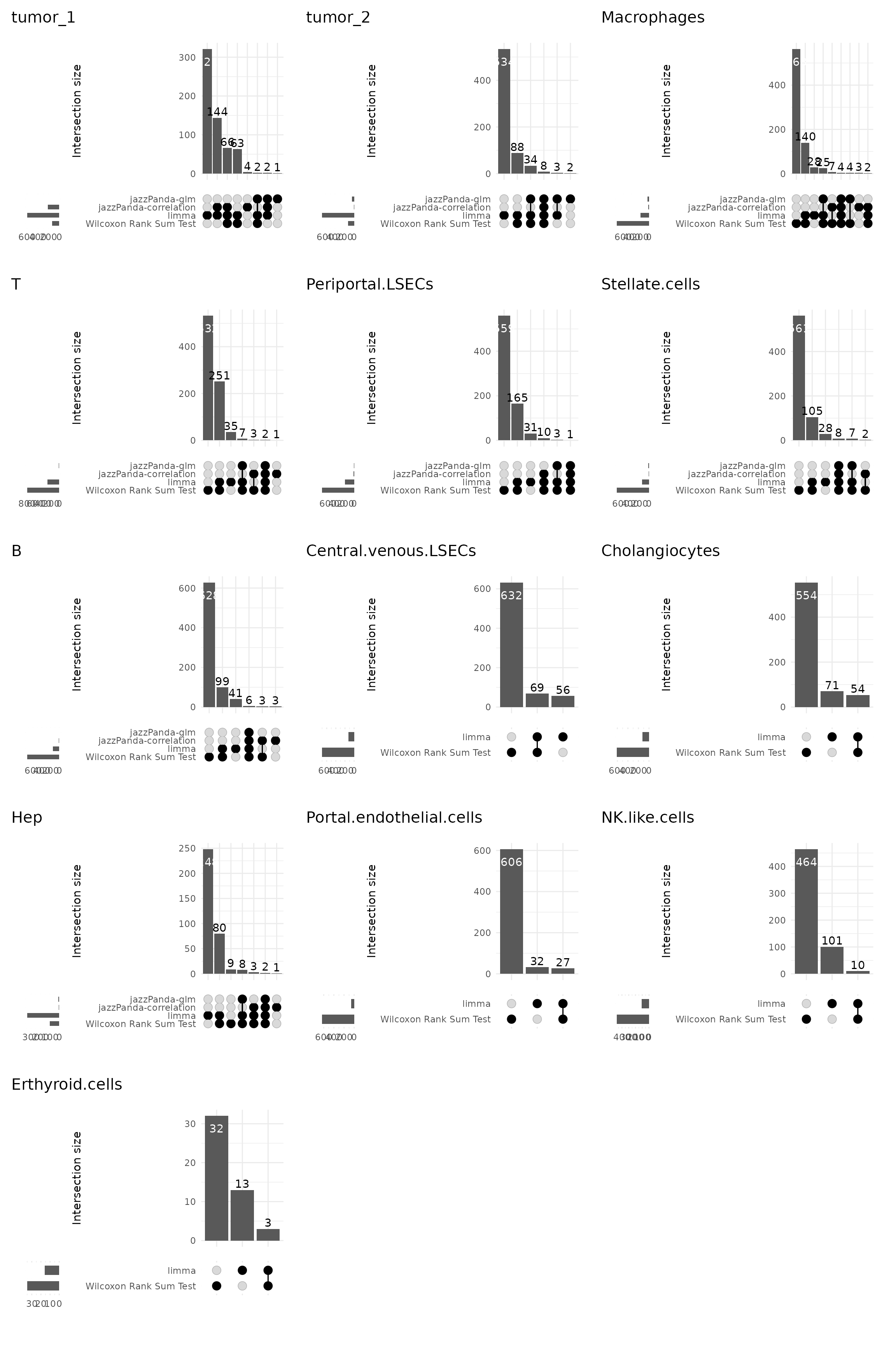
sessionInfo()R version 4.5.1 (2025-06-13)
Platform: x86_64-pc-linux-gnu
Running under: Red Hat Enterprise Linux 9.3 (Plow)
Matrix products: default
BLAS: /stornext/System/data/software/rhel/9/base/tools/R/4.5.1/lib64/R/lib/libRblas.so
LAPACK: /stornext/System/data/software/rhel/9/base/tools/R/4.5.1/lib64/R/lib/libRlapack.so; LAPACK version 3.12.1
locale:
[1] LC_CTYPE=en_AU.UTF-8 LC_NUMERIC=C
[3] LC_TIME=en_AU.UTF-8 LC_COLLATE=en_AU.UTF-8
[5] LC_MONETARY=en_AU.UTF-8 LC_MESSAGES=en_AU.UTF-8
[7] LC_PAPER=en_AU.UTF-8 LC_NAME=C
[9] LC_ADDRESS=C LC_TELEPHONE=C
[11] LC_MEASUREMENT=en_AU.UTF-8 LC_IDENTIFICATION=C
time zone: Australia/Melbourne
tzcode source: system (glibc)
attached base packages:
[1] stats4 stats graphics grDevices utils datasets methods
[8] base
other attached packages:
[1] dotenv_1.0.3 corrplot_0.95
[3] xtable_1.8-4 here_1.0.1
[5] limma_3.64.1 RColorBrewer_1.1-3
[7] patchwork_1.3.1 gridExtra_2.3
[9] ggrepel_0.9.6 ComplexUpset_1.3.3
[11] caret_7.0-1 lattice_0.22-7
[13] glmnet_4.1-10 Matrix_1.7-3
[15] tidyr_1.3.1 dplyr_1.1.4
[17] data.table_1.17.8 ggplot2_3.5.2
[19] Seurat_5.3.0 SeuratObject_5.1.0
[21] sp_2.2-0 SpatialExperiment_1.18.1
[23] SingleCellExperiment_1.30.1 SummarizedExperiment_1.38.1
[25] Biobase_2.68.0 GenomicRanges_1.60.0
[27] GenomeInfoDb_1.44.2 IRanges_2.42.0
[29] S4Vectors_0.46.0 BiocGenerics_0.54.0
[31] generics_0.1.4 MatrixGenerics_1.20.0
[33] matrixStats_1.5.0 jazzPanda_0.2.4
loaded via a namespace (and not attached):
[1] RcppAnnoy_0.0.22 splines_4.5.1 later_1.4.2
[4] tibble_3.3.0 polyclip_1.10-7 hardhat_1.4.2
[7] pROC_1.19.0.1 rpart_4.1.24 fastDummies_1.7.5
[10] lifecycle_1.0.4 rprojroot_2.1.0 globals_0.18.0
[13] MASS_7.3-65 magrittr_2.0.3 plotly_4.11.0
[16] sass_0.4.10 rmarkdown_2.29 jquerylib_0.1.4
[19] yaml_2.3.10 httpuv_1.6.16 sctransform_0.4.2
[22] spam_2.11-1 spatstat.sparse_3.1-0 reticulate_1.43.0
[25] cowplot_1.2.0 pbapply_1.7-4 lubridate_1.9.4
[28] abind_1.4-8 Rtsne_0.17 presto_1.0.0
[31] purrr_1.1.0 BumpyMatrix_1.16.0 nnet_7.3-20
[34] ipred_0.9-15 lava_1.8.1 GenomeInfoDbData_1.2.14
[37] irlba_2.3.5.1 listenv_0.9.1 spatstat.utils_3.1-5
[40] goftest_1.2-3 RSpectra_0.16-2 spatstat.random_3.4-1
[43] fitdistrplus_1.2-4 parallelly_1.45.1 codetools_0.2-20
[46] DelayedArray_0.34.1 tidyselect_1.2.1 shape_1.4.6.1
[49] UCSC.utils_1.4.0 farver_2.1.2 spatstat.explore_3.5-2
[52] jsonlite_2.0.0 progressr_0.15.1 ggridges_0.5.6
[55] survival_3.8-3 iterators_1.0.14 systemfonts_1.3.1
[58] foreach_1.5.2 tools_4.5.1 ragg_1.5.0
[61] ica_1.0-3 Rcpp_1.1.0 glue_1.8.0
[64] prodlim_2025.04.28 SparseArray_1.8.1 xfun_0.52
[67] withr_3.0.2 fastmap_1.2.0 digest_0.6.37
[70] timechange_0.3.0 R6_2.6.1 mime_0.13
[73] textshaping_1.0.1 colorspace_2.1-1 scattermore_1.2
[76] tensor_1.5.1 spatstat.data_3.1-8 hexbin_1.28.5
[79] recipes_1.3.1 class_7.3-23 httr_1.4.7
[82] htmlwidgets_1.6.4 S4Arrays_1.8.1 uwot_0.2.3
[85] ModelMetrics_1.2.2.2 pkgconfig_2.0.3 gtable_0.3.6
[88] timeDate_4041.110 lmtest_0.9-40 XVector_0.48.0
[91] htmltools_0.5.8.1 dotCall64_1.2 scales_1.4.0
[94] png_0.1-8 gower_1.0.2 spatstat.univar_3.1-4
[97] knitr_1.50 reshape2_1.4.4 rjson_0.2.23
[100] nlme_3.1-168 cachem_1.1.0 zoo_1.8-14
[103] stringr_1.5.1 KernSmooth_2.23-26 parallel_4.5.1
[106] miniUI_0.1.2 pillar_1.11.0 grid_4.5.1
[109] vctrs_0.6.5 RANN_2.6.2 promises_1.3.3
[112] cluster_2.1.8.1 evaluate_1.0.4 magick_2.8.7
[115] cli_3.6.5 compiler_4.5.1 rlang_1.1.6
[118] crayon_1.5.3 future.apply_1.20.0 labeling_0.4.3
[121] plyr_1.8.9 stringi_1.8.7 viridisLite_0.4.2
[124] deldir_2.0-4 BiocParallel_1.42.1 lazyeval_0.2.2
[127] spatstat.geom_3.5-0 RcppHNSW_0.6.0 future_1.67.0
[130] statmod_1.5.0 shiny_1.11.1 ROCR_1.0-11
[133] igraph_2.1.4 bslib_0.9.0