How to Prepare Data for SuperCellCyto
Givanna Putri
Source:vignettes/how_to_prepare_data.Rmd
how_to_prepare_data.RmdPerforming Quality Control
Prior to creating supercells, it’s crucial to ensure that your dataset has undergone thorough quality control (QC). We want to retain only single, live cells and remove any debris, doublets, or dead cells. Additionally, it is also important to perform compensation to correct for fluorescence spillover (for Flow data) or to adjust for signal overlap or spillover between different metal isotopse (for Cytof data). A well-prepared dataset is key to obtaining reliable supercells from SuperCellCyto.
Several R packages are available for performing QC on cytometry data. Notable among these are PeacoQC, CATALYST, and CytoExploreR. These packages are well maintained and are continuously updated. To make sure that the information we provide do not quickly go out of date, we highly recommend you to consult the packages’ respective vignettes for detailed guidance on how to use them to QC your data.
In our manuscript, we used CytoExploreR to QC the
Oetjen_bcell flow cytometry data and CATALYST
to QC the Trussart_cytofruv Cytof data.
The specific scripts used can be found in Github:
-
b_cell_identification/gate_flow_data.RforOetjen_bcelldata. -
batch_correction/prepare_data.RforTrussart_cytofruvdata. These scripts were adapted from those used in the CytofRUV manuscript.
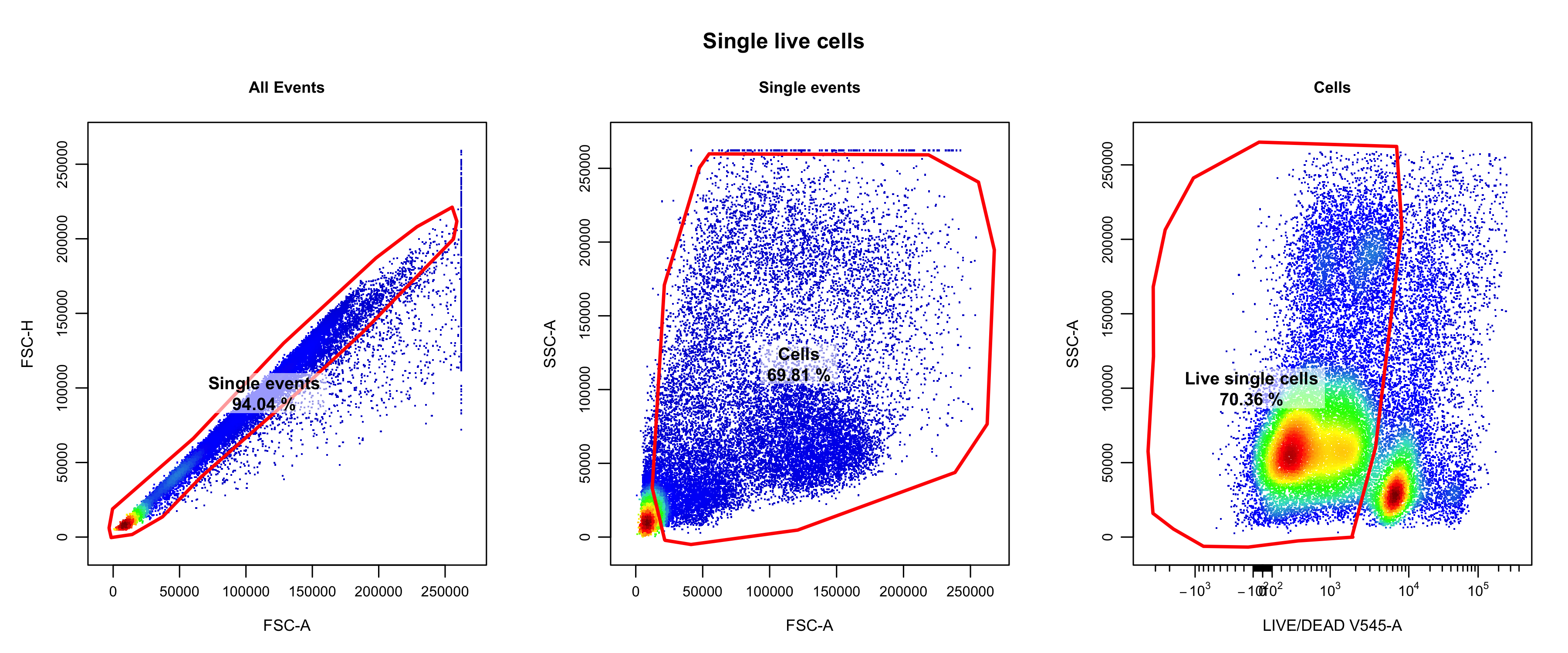
For Oetjen_bcell data, we used the following gating strategy post compensation:
- FSC-H and FSC-A to isolate only the single events. (Also check SSC-H vs SSC-A).
- FSC-A and SSC-A to remove debris.
- Live/Dead and SSC-A to isolate live cells.
The following is the resulting single live cells manually gated for
the Oetjen_bcell data.
knitr::include_graphics(
    "figures/oetjen_bcell_single_live_cells.png",
    error = FALSE
)
After completing the QC process, you will have clean data in either CSV or FCS file formats. The next section will guide you on how to load these files and proceed with preparing your data for SuperCellCyto.
Preparing FCS/CSV files for SuperCellCyto
To use SuperCellCyto, your input data must be formatted as a data.table
object. Briefly, data.table is an enhanced version of R
native data.frame object. It is a package that offers fast
processing of large data.frame.
Cell ID column
Additionally, each cell in your data.table must also
have a unique identifier. The purpose of this ID is to allow SuperCell
to uniquely identify each cell in the dataset. It will come in super
handy later when/if we need to work out which cells belong to which
supercells, i.e., when we need to expand the supercells out. Generally,
we will need to create this ID ourselves. Most dataset won’t come with
this ID already embedded in.
For this tutorial, we will call the column that denotes the cell ID cell_id. For your own dataset, you can name this column however you like, e.g., id, cell_identity, etc. Just make sure you note the column name as we will need it later to create supercells.
Sample column
Lastly, each cell in the data.table object must also be
associated with a sample. This information must be stored in a column
that we later on pass to the function that creates supercells.
Generally, sample here typically refers to the biological sample the
cell came from.
To create supercells, it is necessary to have this column in our dataset. This is to ensure that each supercell will only have cells from exactly one sample. In most cases, it does not make sense to mix cells from different biological samples in one supercell. Additionally (not as important), SuperCellCyto can process multiple samples in parallel, and for it to do that, it needs to know the sample information.
But what if we only have 1 biological sample in our dataset? It does not matter. We still need to have the sample column in our dataset. The only difference is that this column will only have 1 unique value.
You can name the column however we like, e.g., Samp, Cell_Samp, etc. For this tutorial, we will call the column sample. Just make sure you note the column name as we will need it later to create supercells.
Preparing CSV files
Loading CSV files into a data.table object is
straightforward. We can use the fread function from the
data.table package.
For this example, let’s load two CSV files containing subsampled data
from the Levine_32dim dataset we used in SuperCellCyto
manuscript. Each file represents a sample (H1 and H2), with the sample
name appended to the file name:
library(data.table)

csv_files <- system.file(
    "extdata",
    c("Levine_32dim_H1_sub.csv", "Levine_32dim_H2_sub.csv"),
    package = "SuperCellCyto"
)

samples <- c("H1", "H2")

dat <- lapply(seq_len(length(samples)), function(i) {
    csv_file <- csv_files[i]
    sample <- samples[i]

    dat_a_sample <- fread(csv_file)
    dat_a_sample$sample <- sample

    return(dat_a_sample)
})
dat <- rbindlist(dat)

dat[, cell_id := paste0("Cell_", seq_len(nrow(dat)))]

head(dat)
#>      Time Cell_length      DNA1     DNA2   CD45RA      CD133       CD19
#>     <num>       <int>     <num>    <num>    <num>      <num>      <num>
#> 1: 307428          27 169.91125 262.3192 2.338830 -0.1533398 -0.2056334
#> 2:  80712          13  50.91230 181.1320 2.129232  3.3563867 -0.1013980
#> 3: 284190          53  98.28069 187.2090 4.289627  0.5625419 12.2265682
#> 4: 324301          25  94.70678 258.6657 6.537235  0.3936968 37.9688492
#> 5: 253799          45  76.75870 128.8098 4.390123  0.3281800  0.3218679
#> 6: 313897          50 156.23492 254.4634 4.722823  1.5105748 -0.2037212
#>          CD22     CD11b         CD4          CD8        CD34        Flt3
#>         <num>     <num>       <num>        <num>       <num>       <num>
#> 1: -0.1972007 32.130402  0.78105438 -0.071934469  1.53498471  0.84833205
#> 2:  3.0564795 14.239288  0.53373063 -0.007943562 -0.09401329 -0.13234507
#> 3: 10.8176870  1.826709  1.30010796 -0.187664956  2.05419374  2.72891521
#> 4: 22.7653027  0.176247 -0.04688064 -0.075562298  3.77700782  0.01351853
#> 5:  2.2320855  1.343770  2.38195324 -0.120859891 -0.01110659  2.28398013
#> 6:  1.3113755 32.728638  0.33130702 -0.073869787  1.14790535  0.23651542
#>            CD20     CXCR4    CD235ab      CD45       CD123     CD321
#>           <num>     <num>      <num>     <num>       <num>     <num>
#> 1: -0.086762585  3.488938  0.8230118  313.8038  0.30909532 46.484669
#> 2: -0.042171009  1.364644 -0.1309417  207.2459  1.76594567 22.532978
#> 3: 15.341629982  9.303430  6.3413548  751.0563  0.05031190 10.463912
#> 4: 48.562511444 26.948063  0.2169415  588.5150  2.96119761 22.149944
#> 5:  3.535085201  2.498724 12.1216116 1007.4561 -0.18679842  5.777249
#> 6: -0.003814452  6.879488  4.4369431  918.5178 -0.03130747 24.542976
#>           CD14        CD33     CD47      CD11c          CD7      CD15
#>          <num>       <num>    <num>      <num>        <num>     <num>
#> 1:  0.05072345  2.09802437 20.96871 20.7631855 -0.007966662 0.7279212
#> 2: -0.19256826  7.35230541 27.49848 15.1339817 -0.087256350 0.7187206
#> 3:  1.11993504  0.15872155 40.63973  4.6401038 -0.195279136 4.5712810
#> 4: -0.17467052 -0.18741834  7.64338 -0.1591413  0.604379535 1.1375968
#> 5: -0.20860019  0.04116142 30.60899  1.8959216 39.631023407 0.8820186
#> 6:  0.64118510  2.93926096 18.20175 34.3703728 -0.016664671 1.1723862
#>           CD16      CD44      CD38        CD13         CD3       CD61
#>          <num>     <num>     <num>       <num>       <num>      <num>
#> 1: -0.03067662  95.71002  5.112477  5.10564327   0.5827813 -0.1684093
#> 2:  0.41139653 185.51929  7.478415  0.35808861   1.8861074  1.9233229
#> 3: -0.10192144  98.09428 43.535297  2.83275175   0.1868679  2.1032026
#> 4:  1.02131248  45.03027  3.396393 -0.09499715   0.8835158  5.2639704
#> 5:  0.28814790  81.63257  8.634666  0.80971009 728.0478516  1.9550949
#> 6:  2.46474814 250.00719 17.964558  0.38511425   1.4373373  9.9041309
#>          CD117     CD49d      HLA-DR       CD64        CD41 Viability
#>          <num>     <num>       <num>      <num>       <num>     <num>
#> 1: -0.02967962  6.557199 112.4675446  6.9157209  0.08380865  1.726863
#> 2: -0.14122920  1.088500  12.2067947 30.7242870  7.75372791  3.712019
#> 3:  0.01776284 12.400333 174.9526672  0.4361930  1.83412540 13.274319
#> 4:  0.19813232  2.382564   3.4147604  0.9252884 -0.06184266  1.482011
#> 5:  3.34092522  1.395274   0.3110902  0.1227915  0.27702999  3.165646
#> 6:  0.46414420 14.136827  26.3479862 20.1809521 10.70872402 23.840090
#>    file_number event_number sample cell_id
#>          <int>        <int> <char>  <char>
#> 1:          94       257088     H1  Cell_1
#> 2:          94        80655     H1  Cell_2
#> 3:          94       241699     H1  Cell_3
#> 4:          94       268117     H1  Cell_4
#> 5:          94       221804     H1  Cell_5
#> 6:          94       261282     H1  Cell_6
Let’s break down what we have done.
We specify the location of the csv files in csv_files
vector and their corresponding sample names in samples
vector. Levine_32dim_H1_sub.csv belongs to sample H1 while
Levine_32dim_H2_sub.csv belongs to sample H2.
We use lapply to simultaneously iterate over each
element in the csv_files and samples vector.
For each csv file and the corresponding sample, we read the csv file
into the variable dat_a_sample using fread
function. We then assign the sample id in a new column called
sample. As a result, we get a list dat
containing 2 data.table objects, 1 object per csv file.
We use rbindlist function from the
data.table package to merge list into one
data.table object.
We create a new column cell_id which gives each cell a
unique id such as Cell_1, Cell_2, etc.
Preparing FCS files
FCS files, commonly used in cytometry, require specific handling. You
can read in FCS files using the flowCore package available
from Bioconductor and convert it to a data.table
object.
Let’s load two small FCS files for the Anti-PD1 data from FlowRepository.
library(flowCore)
library(data.table)

fs <- read.flowSet(
    path = system.file(
        "extdata",
        package = "SuperCellCyto"
    ),
    pattern = "\\.fcs$"
)

dat_list <- lapply(seq_along(fs), function(i) {
    df <- as.data.table(exprs(fs[[i]]))

    # concatenate channel and marker name as column names
    names(df) <- markernames(fs[[i]])

    # add a column showing the filename
    df$file_name <- sampleNames(fs)[i]

    return(df)
})

# collate all the files into one
dat <- rbindlist(dat_list)

dat
#>      209Bi_CD11b 162Dy_CD11c  163Dy_CD7 166Er_CD209  167Er_CD38 151Eu_CD123
#>            <num>       <num>      <num>       <num>       <num>       <num>
#>   1:    2.596444    0.000000  24.233248   2.4271879   0.2497845  0.01359761
#>   2:   20.172476   29.508638 253.930161   2.0283859  63.4845619  0.00000000
#>   3:  224.771057  377.262421  20.755060   5.5264821 111.7728882 10.33144855
#>   4:  711.252808  192.961227  16.039482   2.7453365  13.4806919  1.71946943
#>   5:  435.131073  203.836838   5.983910   0.0000000   4.2271118  1.08193946
#>  ---
#> 569:  337.737152  160.982407   1.724550   0.8164008  10.8179998  1.87148142
#> 570:   48.965187    3.454711  55.719162   0.7539494  20.6741104  0.00000000
#> 571:  326.666168   58.792435   4.358847   0.0000000   8.6697922  0.00000000
#> 572:    7.255682    0.000000   3.552515   0.0000000   2.9367595  0.43651727
#> 573:  349.350769   31.072611   1.050743   0.0000000   5.4545450  5.87748337
#>      153Eu_CD62L 152Gd_CD66b 154Gd_ICAM-1 155Gd_CD1c  156Gd_CD86 160Gd_CD14
#>            <num>       <num>        <num>      <num>       <num>      <num>
#>   1:  276.736237   0.0000000    6.3661394 0.72167069   0.0000000   0.000000
#>   2:    7.522890   0.0000000   16.6949806 0.00000000   0.9723848   2.370285
#>   3:    2.523962   0.0000000  480.9555969 2.87207913 109.6869812  41.803619
#>   4:    1.439798   0.0000000  125.3002014 0.00000000   5.1308088  19.226034
#>   5:    3.030660   0.0000000   54.1368217 0.03324713  23.3382854  14.204736
#>  ---
#> 569:    0.000000   0.0000000  158.1088257 2.28826094  15.2002096   5.657256
#> 570:    3.414483   0.0000000    0.9569107 2.11766744   0.7849152   4.082072
#> 571:    0.000000   0.0000000    1.1182016 0.00000000   0.0000000   0.000000
#> 572:    2.556602   0.6154923    0.0000000 0.00000000   0.0000000   0.000000
#> 573:    3.925082   0.0000000   43.5083618 0.00000000   4.2216253   8.216695
#>       165Ho_CD16 191Ir_DNA1 193Ir_DNA2 175Lu_PD-L1 142Nd_CD19 146Nd_CD64
#>            <num>      <num>      <num>       <num>      <num>      <num>
#>   1:   0.0000000   40.33384   76.70573   0.0000000 0.00000000   5.452389
#>   2: 126.4256592   55.11267  150.46278   3.4527724 0.00000000   1.922374
#>   3:   2.0556698   91.42932  161.59381   8.3969393 0.00000000  12.956987
#>   4:   0.0000000   75.32122  160.41399   0.1078656 0.00000000  12.841355
#>   5:   0.5523136   79.88800  142.12471   0.6882498 0.00000000  19.308508
#>  ---
#> 569:   0.0000000   65.31769  148.84435   0.1064020 0.00000000  22.941177
#> 570:  51.3577194   65.16866  129.46790   3.5496852 0.36609724   2.852356
#> 571:   0.9855582   92.97505  151.65977   0.0000000 0.03485066   6.290884
#> 572:   0.0000000   65.07745  111.99138   0.5479890 0.63119560   0.000000
#> 573:   0.0000000  114.67633  191.50166   0.0000000 0.00000000  12.638340
#>          195Pt     196Pt 198Pt_Dead 147Sm_CD303 148Sm_CD34 149Sm_CD141
#>          <num>     <num>      <num>       <num>      <num>       <num>
#>   1: 0.0000000 0.0000000  15.199163   0.0000000  1.2188276    2.482402
#>   2: 2.6318610 0.0000000  32.325874   0.0000000  0.2467884    0.000000
#>   3: 0.2854315 0.3602256  10.119688   0.7021694  7.2453775   17.055792
#>   4: 1.7483448 1.6977243   2.457203   0.0000000  1.1050161    6.811901
#>   5: 0.0000000 2.7839208  13.680239   0.8908378  0.0000000   18.400421
#>  ---
#> 569: 0.0000000 0.0000000  16.751446   2.6801469  0.6307272    2.710867
#> 570: 0.3765990 0.0000000  20.695446   0.0000000  3.0734873    1.968072
#> 571: 0.1897834 0.0000000  16.076082   0.9444249  0.4878764    6.945232
#> 572: 0.0000000 0.0000000  23.279974   0.0000000  0.0000000    0.000000
#> 573: 0.0000000 4.0132923  12.463143   0.8065992  1.6200637    4.190233
#>      150Sm_CD61  169Tm_CD33  89Y_CD45  170Yb_CD3  173Yb_CD56 174Yb_HLA-DR
#>           <num>       <num>     <num>      <num>       <num>        <num>
#>   1:  65.015724   1.1326860  37.52760  9.0316811  0.00000000     6.807954
#>   2:  25.455738   0.1979908 225.64279  0.9135754  8.38446426     5.601559
#>   3:  75.056625 134.7255249 458.79022 12.2988071 10.31508160   403.328308
#>   4:  21.287003  58.7627487 387.78836  1.1870043  0.00000000    88.822212
#>   5:  26.795689  35.0521393 107.94828  0.3782265  5.60699320   104.159081
#>  ---
#> 569:  36.163387  22.8519592 227.01973  2.7277973  0.02519703   188.378601
#> 570:  37.537052   3.3848262  48.12588  4.6816015  2.54012346    10.622149
#> 571:  16.739002  10.3474064  60.64515  0.6677586  0.00000000    15.465885
#> 572:  15.469506   0.0000000  11.47586  8.9600000  0.00000000     0.000000
#> 573:   8.587144  18.8689251  52.50787  0.6892268  1.88265443    13.542062
#>                                file_name
#>                                   <char>
#>   1: Data23_Panel3_base_NR4_Patient9.fcs
#>   2: Data23_Panel3_base_NR4_Patient9.fcs
#>   3: Data23_Panel3_base_NR4_Patient9.fcs
#>   4: Data23_Panel3_base_NR4_Patient9.fcs
#>   5: Data23_Panel3_base_NR4_Patient9.fcs
#>  ---
#> 569: Data23_Panel3_base_R5_Patient15.fcs
#> 570: Data23_Panel3_base_R5_Patient15.fcs
#> 571: Data23_Panel3_base_R5_Patient15.fcs
#> 572: Data23_Panel3_base_R5_Patient15.fcs
#> 573: Data23_Panel3_base_R5_Patient15.fcs
The code above used flowCore’s read.flowSet
function to first read FCS files into a flowSet object.
lapply and rbindlist is then used to
convert it to one data.table object containing data from
all FCS files.
The FCS files belong to two different patients, patient 9 and 15. We
shall use that as the sample ID. To make sure that we correctly map the
filenames to the patients, we will first create a new
data.table object containing the mapping of FileName and
the sample name, and then using merge.data.table to add
them into our data.table object.
We will also to create a new column cell_id which gives
each cell a unique id such as Cell_1, Cell_2,
etc.
sample_info <- data.table(
    sample = c("patient9", "patient15"),
    file_name = c(
        "Data23_Panel3_base_NR4_Patient9.fcs",
        "Data23_Panel3_base_R5_Patient15.fcs"
    )
)
dat <- merge.data.table(
    x = dat,
    y = sample_info,
    by = "file_name"
)

dat[, cell_id := paste0("Cell_", seq_len(nrow(dat)))]
With CSV and FCS files loaded as data.table objects, the next step is to transform the data appropriately for SuperCellCyto.
Data Transformation
Before using SuperCellCyto, it’s essential to apply appropriate data transformations.
A common method for data transformation in cytometry is the arcsinh transformation, an inverse hyperbolic arcsinh transformation. The transformation requires specifying a cofactor, which affects the representation of the low-end data. Typically, a cofactor of 5 is used for Cytof data and 150 for Flow data. This vignette will focus on the transformation process rather than cofactor selection.
We’ll use the Levine_32dim dataset loaded earlier from
CSV files.
First, we need to select the markers to be transformed. Usually, all markers should be transformed for SuperCellCyto. However, you can choose to exclude specific markers if needed:
markers <- c(
    "209Bi_CD11b", "162Dy_CD11c", "163Dy_CD7", "166Er_CD209", "167Er_CD38",
    "151Eu_CD123", "153Eu_CD62L", "152Gd_CD66b", "154Gd_ICAM-1", "155Gd_CD1c",
    "156Gd_CD86", "160Gd_CD14", "165Ho_CD16", "191Ir_DNA1", "193Ir_DNA2",
    "175Lu_PD-L1", "142Nd_CD19", "146Nd_CD64", "195Pt", "196Pt",
    "198Pt_Dead", "147Sm_CD303", "148Sm_CD34", "149Sm_CD141", "150Sm_CD61",
    "169Tm_CD33", "89Y_CD45", "170Yb_CD3", "173Yb_CD56", "174Yb_HLA-DR"
)
For transformation, we’ll use a cofactor of 5 and apply the arcsinh transformation.
new_cols <- paste0(markers, "_asinh")
cf <- 5
dat[, (new_cols) := lapply(.SD, function(x) asinh(x / cf)), .SDcols = markers]
After transformation, new columns with “_asinh” appended indicate the transformed markers.
head(dat)
#> Key: <file_name>
#>                              file_name 209Bi_CD11b 162Dy_CD11c  163Dy_CD7
#>                                 <char>       <num>       <num>      <num>
#> 1: Data23_Panel3_base_NR4_Patient9.fcs    2.596444     0.00000  24.233248
#> 2: Data23_Panel3_base_NR4_Patient9.fcs   20.172476    29.50864 253.930161
#> 3: Data23_Panel3_base_NR4_Patient9.fcs  224.771057   377.26242  20.755060
#> 4: Data23_Panel3_base_NR4_Patient9.fcs  711.252808   192.96123  16.039482
#> 5: Data23_Panel3_base_NR4_Patient9.fcs  435.131073   203.83684   5.983910
#> 6: Data23_Panel3_base_NR4_Patient9.fcs  182.881317   244.65285   5.262897
#>    166Er_CD209  167Er_CD38 151Eu_CD123 153Eu_CD62L 152Gd_CD66b 154Gd_ICAM-1
#>          <num>       <num>       <num>       <num>       <num>        <num>
#> 1:    2.427188   0.2497845  0.01359761  276.736237           0     6.366139
#> 2:    2.028386  63.4845619  0.00000000    7.522890           0    16.694981
#> 3:    5.526482 111.7728882 10.33144855    2.523962           0   480.955597
#> 4:    2.745337  13.4806919  1.71946943    1.439798           0   125.300201
#> 5:    0.000000   4.2271118  1.08193946    3.030660           0    54.136822
#> 6:    1.548412  34.4840889  1.36238360    0.000000           0    13.646034
#>    155Gd_CD1c  156Gd_CD86 160Gd_CD14  165Ho_CD16 191Ir_DNA1 193Ir_DNA2
#>         <num>       <num>      <num>       <num>      <num>      <num>
#> 1: 0.72167069   0.0000000   0.000000   0.0000000   40.33384   76.70573
#> 2: 0.00000000   0.9723848   2.370285 126.4256592   55.11267  150.46278
#> 3: 2.87207913 109.6869812  41.803619   2.0556698   91.42932  161.59381
#> 4: 0.00000000   5.1308088  19.226034   0.0000000   75.32122  160.41399
#> 5: 0.03324713  23.3382854  14.204736   0.5523136   79.88800  142.12471
#> 6: 4.62103748  11.6817465   2.560833   0.0000000   56.35513   93.84315
#>    175Lu_PD-L1 142Nd_CD19 146Nd_CD64     195Pt     196Pt 198Pt_Dead 147Sm_CD303
#>          <num>      <num>      <num>     <num>     <num>      <num>       <num>
#> 1:   0.0000000          0   5.452389 0.0000000 0.0000000  15.199163   0.0000000
#> 2:   3.4527724          0   1.922374 2.6318610 0.0000000  32.325874   0.0000000
#> 3:   8.3969393          0  12.956987 0.2854315 0.3602256  10.119688   0.7021694
#> 4:   0.1078656          0  12.841355 1.7483448 1.6977243   2.457203   0.0000000
#> 5:   0.6882498          0  19.308508 0.0000000 2.7839208  13.680239   0.8908378
#> 6:   5.6380033          0   8.388703 0.0000000 0.0000000   3.202339   0.7597103
#>    148Sm_CD34 149Sm_CD141 150Sm_CD61  169Tm_CD33 89Y_CD45  170Yb_CD3 173Yb_CD56
#>         <num>       <num>      <num>       <num>    <num>      <num>      <num>
#> 1:  1.2188276    2.482402   65.01572   1.1326860  37.5276  9.0316811   0.000000
#> 2:  0.2467884    0.000000   25.45574   0.1979908 225.6428  0.9135754   8.384464
#> 3:  7.2453775   17.055792   75.05663 134.7255249 458.7902 12.2988071  10.315082
#> 4:  1.1050161    6.811901   21.28700  58.7627487 387.7884  1.1870043   0.000000
#> 5:  0.0000000   18.400421   26.79569  35.0521393 107.9483  0.3782265   5.606993
#> 6:  4.0056577    2.323631   12.82973  55.7610817 444.4799  0.6113114   1.556887
#>    174Yb_HLA-DR   sample cell_id 209Bi_CD11b_asinh 162Dy_CD11c_asinh
#>           <num>   <char>  <char>             <num>             <num>
#> 1:     6.807954 patient9  Cell_1         0.4983974          0.000000
#> 2:     5.601559 patient9  Cell_2         2.1030451          2.475494
#> 3:   403.328308 patient9  Cell_3         4.4989153          5.016694
#> 4:    88.822212 patient9  Cell_4         5.6507496          4.346366
#> 5:   104.159081 patient9  Cell_5         5.1593896          4.401180
#> 6:   145.182190 patient9  Cell_6         4.2927335          4.583654
#>    163Dy_CD7_asinh 166Er_CD209_asinh 167Er_CD38_asinh 151Eu_CD123_asinh
#>              <num>             <num>            <num>             <num>
#> 1:       2.2819117         0.4681490       0.04993614       0.002719519
#> 2:       4.6208655         0.3953013       3.23605319       0.000000000
#> 3:       2.1307022         0.9539050       3.80067819       1.472894089
#> 4:       1.8822162         0.5246630       1.71770981       0.337452783
#> 5:       1.0139113         0.0000000       0.76774561       0.214733831
#> 6:       0.9180684         0.3049346       2.62942218       0.269213018
#>    153Eu_CD62L_asinh 152Gd_CD66b_asinh 154Gd_ICAM-1_asinh 155Gd_CD1c_asinh
#>                <num>             <num>              <num>            <num>
#> 1:         4.7068557                 0           1.062022      0.143837642
#> 2:         1.1972999                 0           1.920522      0.000000000
#> 3:         0.4854943                 0           5.259511      0.546763229
#> 4:         0.2841215                 0           3.914820      0.000000000
#> 5:         0.5740759                 0           3.077350      0.006649377
#> 6:         0.0000000                 0           1.729148      0.826752274
#>    156Gd_CD86_asinh 160Gd_CD14_asinh 165Ho_CD16_asinh 191Ir_DNA1_asinh
#>               <num>            <num>            <num>            <num>
#> 1:        0.0000000        0.0000000        0.0000000         2.784720
#> 2:        0.1932715        0.4578881        3.9237545         3.095140
#> 3:        3.7818590        2.8202496        0.4003530         3.600022
#> 4:        0.8997523        2.0564695        0.0000000         3.406571
#> 5:        2.2450865        1.7669123        0.1102393         3.465313
#> 6:        1.5846764        0.4920673        0.0000000         3.117345
#>    193Ir_DNA2_asinh 175Lu_PD-L1_asinh 142Nd_CD19_asinh 146Nd_CD64_asinh
#>               <num>             <num>            <num>            <num>
#> 1:         3.424746        0.00000000                0        0.9439264
#> 2:         4.097701        0.64491132                0        0.3755822
#> 3:         4.169034        1.29032235                0        1.6806506
#> 4:         4.161710        0.02157144                0        1.6722922
#> 5:         4.040723        0.13721893                0        2.0606128
#> 6:         3.626043        0.96878631                0        1.2894793
#>    195Pt_asinh 196Pt_asinh 198Pt_Dead_asinh 147Sm_CD303_asinh 148Sm_CD34_asinh
#>          <num>       <num>            <num>             <num>            <num>
#> 1:  0.00000000  0.00000000        1.8309680         0.0000000       0.24141372
#> 2:  0.50467458  0.00000000        2.5655054         0.0000000       0.04933766
#> 3:  0.05705535  0.07198295        1.4542897         0.1399763       1.16617935
#> 4:  0.34290908  0.33333742        0.4735430         0.0000000       0.21924260
#> 5:  0.00000000  0.53141631        1.7314988         0.1772382       0.00000000
#> 6:  0.00000000  0.00000000        0.6032147         0.1513634       0.73355159
#>    149Sm_CD141_asinh 150Sm_CD61_asinh 169Tm_CD33_asinh 89Y_CD45_asinh
#>                <num>            <num>            <num>          <num>
#> 1:         0.4780616         3.259814       0.22464301       2.713195
#> 2:         0.0000000         2.330159       0.03958781       4.502785
#> 3:         1.9410230         3.403060       3.98729298       5.212332
#> 4:         1.1159197         2.155322       3.15902249       5.044211
#> 5:         2.0140514         2.380543       2.64559441       3.765897
#> 6:         0.4494416         1.671448       3.10678950       5.180646
#>    170Yb_CD3_asinh 173Yb_CD56_asinh 174Yb_HLA-DR_asinh
#>              <num>            <num>              <num>
#> 1:      1.35351374        0.0000000          1.1154525
#> 2:      0.18171341        1.2890452          0.9639413
#> 3:      1.63218235        1.4714672          5.0834986
#> 4:      0.23522564        0.0000000          3.5711373
#> 5:      0.07557334        0.9646649          3.7302042
#> 6:      0.12195971        0.3065534          4.0619951
With your data now transformed, you’re ready to create supercells using SuperCellCyto. Please refer to How to create supercells vignette for detailed instructions.
Session information
sessionInfo()
#> R version 4.5.1 (2025-06-13)
#> Platform: x86_64-pc-linux-gnu
#> Running under: Ubuntu 24.04.3 LTS
#>
#> Matrix products: default
#> BLAS:   /usr/lib/x86_64-linux-gnu/openblas-pthread/libblas.so.3
#> LAPACK: /usr/lib/x86_64-linux-gnu/openblas-pthread/libopenblasp-r0.3.26.so;  LAPACK version 3.12.0
#>
#> locale:
#>  [1] LC_CTYPE=C.UTF-8       LC_NUMERIC=C           LC_TIME=C.UTF-8
#>  [4] LC_COLLATE=C.UTF-8     LC_MONETARY=C.UTF-8    LC_MESSAGES=C.UTF-8
#>  [7] LC_PAPER=C.UTF-8       LC_NAME=C              LC_ADDRESS=C
#> [10] LC_TELEPHONE=C         LC_MEASUREMENT=C.UTF-8 LC_IDENTIFICATION=C
#>
#> time zone: UTC
#> tzcode source: system (glibc)
#>
#> attached base packages:
#> [1] stats     graphics  grDevices utils     datasets  methods   base
#>
#> other attached packages:
#> [1] flowCore_2.20.0   data.table_1.17.8 BiocStyle_2.36.0
#>
#> loaded via a namespace (and not attached):
#>  [1] cli_3.6.5           knitr_1.50          rlang_1.1.6
#>  [4] xfun_0.53           png_0.1-8           generics_0.1.4
#>  [7] textshaping_1.0.4   jsonlite_2.0.0      RProtoBufLib_2.20.0
#> [10] S4Vectors_0.46.0    htmltools_0.5.8.1   stats4_4.5.1
#> [13] ragg_1.5.0          sass_0.4.10         Biobase_2.68.0
#> [16] rmarkdown_2.30      evaluate_1.0.5      jquerylib_0.1.4
#> [19] fastmap_1.2.0       yaml_2.3.10         lifecycle_1.0.4
#> [22] bookdown_0.45       BiocManager_1.30.26 compiler_4.5.1
#> [25] fs_1.6.6            htmlwidgets_1.6.4   systemfonts_1.3.1
#> [28] digest_0.6.37       R6_2.6.1            cytolib_2.20.0
#> [31] bslib_0.9.0         tools_4.5.1         matrixStats_1.5.0
#> [34] BiocGenerics_0.54.1 pkgdown_2.1.3       cachem_1.1.0
#> [37] desc_1.4.3