Interoperability with SingleCellExperiment

Introduction

This vignette demonstrates how to integrate SuperCellCyto results with cytometry data stored in SingleCellExperiment (SCE) objects, and how to analyse SuperCellCyto output using Bioconductor packages that take SCE objects as input.

We use a subsampled Levine_32dim dataset stored in an SCE object to illustrate how to create supercells and conduct downstream analyses.

library(SuperCellCyto)
library(qs2)
library(scran)
library(BiocSingular)
library(scater)
library(bluster)
library(data.table)

Preparing SCE object

We first load the subsampled Levine_32dim data, stored as a qs2 using the qs_read function.

sce <- qs_read(
    system.file(
        "extdata", 
        "Levine_32dim_sce_sub.qs2", 
        package = "SuperCellCyto"
    )
)
sce
#> class: SingleCellExperiment 
#> dim: 39 1500 
#> metadata(0):
#> assays(1): counts
#> rownames(39): Time Cell_length ... file_number event_number
#> rowData names(0):
#> colnames(1500): cell_1 cell_2 ... cell_1499 cell_1500
#> colData names(3): population sample cell_id
#> reducedDimNames(0):
#> mainExpName: NULL
#> altExpNames(0):

The data is stored in the counts assay. We will subset it to include only markers we need to perform downstream analysis, transform it using arcsinh transformation, and store the transformed data in the logcounts assay.

markers <- c(
    "CD45RA", "CD133", "CD19", "CD22", "CD11b", "CD4", "CD8",
    "CD34", "Flt3", "CD20", "CXCR4", "CD235ab", "CD45", "CD123", "CD321",
    "CD14", "CD33", "CD47", "CD11c", "CD7", "CD15", "CD16", "CD44", "CD38",
    "CD13", "CD3", "CD61", "CD117",
    "CD49d", "HLA-DR", "CD64", "CD41"
)

# keep only the relevant markers
sce <- sce[markers, ]

# to store arcsinh transformed data
exprs(sce) <- asinh(counts(sce) / 5)

sce
#> class: SingleCellExperiment 
#> dim: 32 1500 
#> metadata(0):
#> assays(2): counts logcounts
#> rownames(32): CD45RA CD133 ... CD64 CD41
#> rowData names(0):
#> colnames(1500): cell_1 cell_2 ... cell_1499 cell_1500
#> colData names(3): population sample cell_id
#> reducedDimNames(0):
#> mainExpName: NULL
#> altExpNames(0):

Run SuperCellCyto

SuperCellCyto requires input data in a data.table format. Therefore, we need to extract the arcsinh-transformed data into a data.table object, and add the sample information and IDs of the cells.

Note that SCE typically stores cells as columns and features as rows. SuperCellCyto, conversely, requires cells as rows and features as columns, a format typical for cytometry data where we typically have more cells than features. Hence, we will transpose the extracted data accordingly when creating the data.table object.

dt <- data.table(t(exprs(sce)))
dt$sample <- colData(sce)$sample
dt$cell_id <- colnames(sce)

supercells <- runSuperCellCyto(
    dt = dt,
    markers = markers,
    sample_colname = "sample",
    cell_id_colname = "cell_id",
    gam = 5
)

head(supercells$supercell_expression_matrix)
#>       CD45RA     CD133       CD19        CD22     CD11b        CD4          CD8
#>        <num>     <num>      <num>       <num>     <num>      <num>        <num>
#> 1: 0.7567786 0.2094107 0.07620974 0.009254529 0.3511375 0.78500942 0.8687925975
#> 2: 1.1482748 0.6268151 0.40876592 0.091766210 0.2766514 0.09603202 1.3321355589
#> 3: 0.1700757 0.1339944 0.07228738 0.101802043 0.1040339 0.18761509 0.1132434207
#> 4: 0.8968968 0.2921571 2.22313786 0.450342888 0.4193913 0.23917011 0.1332567931
#> 5: 0.1476499 0.1904578 0.11589638 0.106288009 0.2489399 0.52420384 0.4813924176
#> 6: 0.3801373 0.2772991 0.68028804 0.237641653 0.2007602 0.04097948 0.0001923242
#>          CD34      Flt3        CD20     CXCR4   CD235ab     CD45        CD123
#>         <num>     <num>       <num>     <num>     <num>    <num>        <num>
#> 1: 0.11526045 0.5488327 0.041534679 1.2172962 0.6303494 5.788989  0.070171026
#> 2: 0.12708141 0.0793773 0.053358629 0.3920845 0.5637494 5.785661  0.084488379
#> 3: 3.23152402 0.1749861 0.008712508 0.5421237 0.1212147 3.416994  0.066197760
#> 4: 0.30587619 0.5787963 0.136006539 1.3302008 0.3211722 4.369223  0.698444542
#> 5: 0.05301752 0.3468969 0.092965825 0.2609136 0.5636011 5.684187 -0.003512615
#> 6: 2.13054119 0.1427986 0.005927587 0.5651623 0.1386637 3.051677  0.143230069
#>       CD321       CD14       CD33     CD47     CD11c        CD7      CD15
#>       <num>      <num>      <num>    <num>     <num>      <num>     <num>
#> 1: 1.500236 0.04154518 0.06746186 3.221072 0.2123768 2.28170702 0.2050279
#> 2: 1.656612 0.08216914 0.12675445 2.043989 0.1105668 2.43975076 0.2104722
#> 3: 2.803258 0.02104697 0.17107591 2.657387 0.3190474 0.03814356 0.2649500
#> 4: 2.654545 0.01727268 0.24770161 4.576991 0.4200163 0.09815344 0.3564437
#> 5: 1.466286 0.08933425 0.02555677 2.352106 0.1591512 2.55868425 0.1185639
#> 6: 2.040685 0.09609030 0.35279157 3.578527 0.2416795 0.02281908 0.5117449
#>          CD16     CD44      CD38       CD13        CD3       CD61       CD117
#>         <num>    <num>     <num>      <num>      <num>      <num>       <num>
#> 1: 0.03168278 2.925953 0.6649237 0.09905437 5.10948135 0.05358984 0.281380801
#> 2: 0.10139879 4.354774 1.1550810 0.22855225 0.58614888 0.16057716 0.003634178
#> 3: 0.04358262 2.895200 0.9998574 0.31835180 0.15497706 0.05665786 0.993750340
#> 4: 0.35695241 5.021503 6.2330245 0.64945662 0.17109374 0.18993344 0.082566733
#> 5: 0.08155028 2.924965 0.3143248 0.09534336 4.89098214 0.22921411 0.059164421
#> 6: 0.06652319 2.830727 3.7236044 0.71869068 0.09991223 0.28525846 0.111576001
#>        CD49d    HLA-DR       CD64       CD41 sample           SuperCellId
#>        <num>     <num>      <num>      <num> <char>                <char>
#> 1: 0.3529696 0.1407416 0.09377686 0.07614376     H1 SuperCell_1_Sample_H1
#> 2: 0.8440716 0.2467888 0.18515576 0.28544083     H1 SuperCell_2_Sample_H1
#> 3: 1.0233080 1.6318626 0.25253230 0.04277276     H1 SuperCell_3_Sample_H1
#> 4: 1.5830615 0.0820442 0.03792944 0.16956875     H1 SuperCell_4_Sample_H1
#> 5: 0.3508159 0.1748238 0.11055986 0.04522353     H1 SuperCell_5_Sample_H1
#> 6: 1.6866826 3.0233062 0.13634514 0.40852578     H1 SuperCell_6_Sample_H1

We can now embed the supercell ID in the colData of our SCE object.

colData(sce)$supercell_id <-  factor(supercells$supercell_cell_map$SuperCellID)
head(colData(sce))
#> DataFrame with 6 rows and 4 columns
#>        population   sample     cell_id            supercell_id
#>          <factor> <factor> <character>                <factor>
#> cell_1  Basophils       H1      cell_1 SuperCell_22_Sample_H1 
#> cell_2  Basophils       H1      cell_2 SuperCell_50_Sample_H1 
#> cell_3  Basophils       H1      cell_3 SuperCell_28_Sample_H1 
#> cell_4  Basophils       H1      cell_4 SuperCell_141_Sample_H1
#> cell_5  Basophils       H1      cell_5 SuperCell_141_Sample_H1
#> cell_6  Basophils       H1      cell_6 SuperCell_99_Sample_H1

Analyse Supercells as SCE object

As the number of supercells is less than the number of cells in our SCE object, we store the supercell expression matrix as a separate SCE object. This then allows us to use Bioconductor packages to analyse our supercells.

supercell_sce <- SingleCellExperiment(
    list(logcounts = t(
        supercells$supercell_expression_matrix[, markers, with = FALSE]
    )),
    colData = DataFrame(
        SuperCellId = supercells$supercell_expression_matrix$SuperCellId,
        sample = supercells$supercell_expression_matrix$sample
    )
)
colnames(supercell_sce) <- colData(supercell_sce)$SuperCellId
supercell_sce
#> class: SingleCellExperiment 
#> dim: 32 300 
#> metadata(0):
#> assays(1): logcounts
#> rownames(32): CD45RA CD133 ... CD64 CD41
#> rowData names(0):
#> colnames(300): SuperCell_1_Sample_H1 SuperCell_2_Sample_H1 ...
#>   SuperCell_149_Sample_H2 SuperCell_150_Sample_H2
#> colData names(2): SuperCellId sample
#> reducedDimNames(0):
#> mainExpName: NULL
#> altExpNames(0):

The code above essentially transpose the supercell expression matrix, making supercells columns and markers rows, and store it in the logcounts assay of our new SCE object. We also populate the colData with SuperCellId and the sample name for each supercell.

With the supercell expression matrix now in an SCE format, we can perform downstream analyses such as clustering and and drawing UMAP plots using Bioconductor packages.

set.seed(42)

supercell_sce <- fixedPCA(
    supercell_sce,
    rank = 10,
    subset.row = NULL,
    BSPARAM = RandomParam()
)
supercell_sce <- runUMAP(supercell_sce, dimred = "PCA")

clusters <- clusterCells(
    supercell_sce, use.dimred = "PCA",
    BLUSPARAM = SNNGraphParam(cluster.fun = "leiden")
)

colLabels(supercell_sce) <- clusters

plotReducedDim(supercell_sce, dimred = "UMAP", colour_by = "label")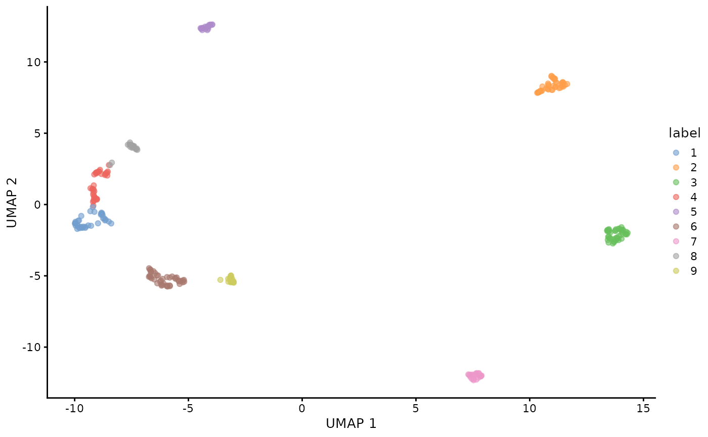

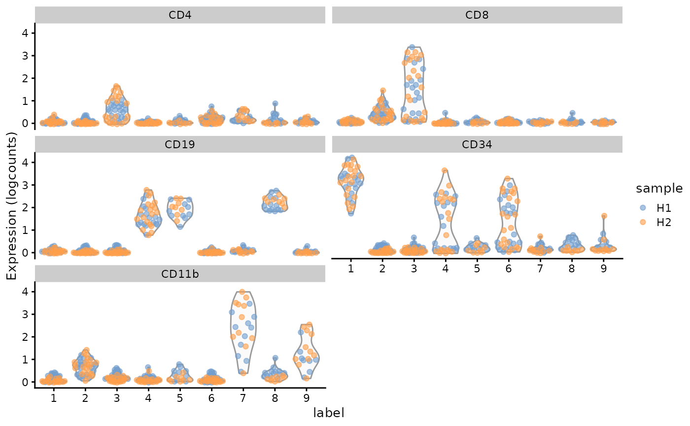
Any functions which operate on SCE object should work. For example, we can use plotExpression in scater package to create violin plots of the markers against clusters.

Note, the y-axis says “logcounts”, but the data is actually arcsinh transformed, not log transformed.

plotExpression(
    supercell_sce, c("CD4", "CD8", "CD19", "CD34", "CD11b"),
    x = "label", colour_by = "sample"
)

Transfer information from supercells SCE object to single cell SCE object

To transfer analysis results (e.g., clusters) from the supercell SCE object back to the single-cell SCE object, we need to do some data wrangling. It is vital to ensure that the order of the analysis results (e.g., clusters) aligns with the cell order in the SCE object.

Using the cluster information as an example, we need to first extract the colData of the SCE objects into two separate data.table objects. We then use merge.data.table to match and merge them using the supercell ID as the common identifiers. Make sure you set the sort parameter to FALSE and set x to the colData of your single cell SCE object. This ensures that the order of the resulting data.table aligns with the order of the colData of our single-cell SCE object.

cell_id_sce <- data.table(as.data.frame(colData(sce)))
supercell_cluster <- data.table(as.data.frame(colData(supercell_sce)))
cell_id_sce_with_clusters <- merge.data.table(
    x = cell_id_sce,
    y = supercell_cluster,
    by.x = "supercell_id",
    by.y = "SuperCellId",
    sort = FALSE
)

Finally, we can then add the cluster assignment as a column in the colData of our single-cell SCE object.

colData(sce)$cluster <- cell_id_sce_with_clusters$label

Visualise them as UMAP plot.

sce <- fixedPCA(sce, rank = 10, subset.row = NULL, BSPARAM = RandomParam())
sce <- runUMAP(sce, dimred = "PCA")

plotReducedDim(sce, dimred = "UMAP", colour_by = "cluster")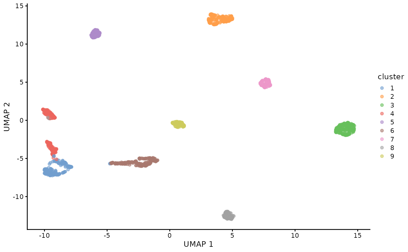

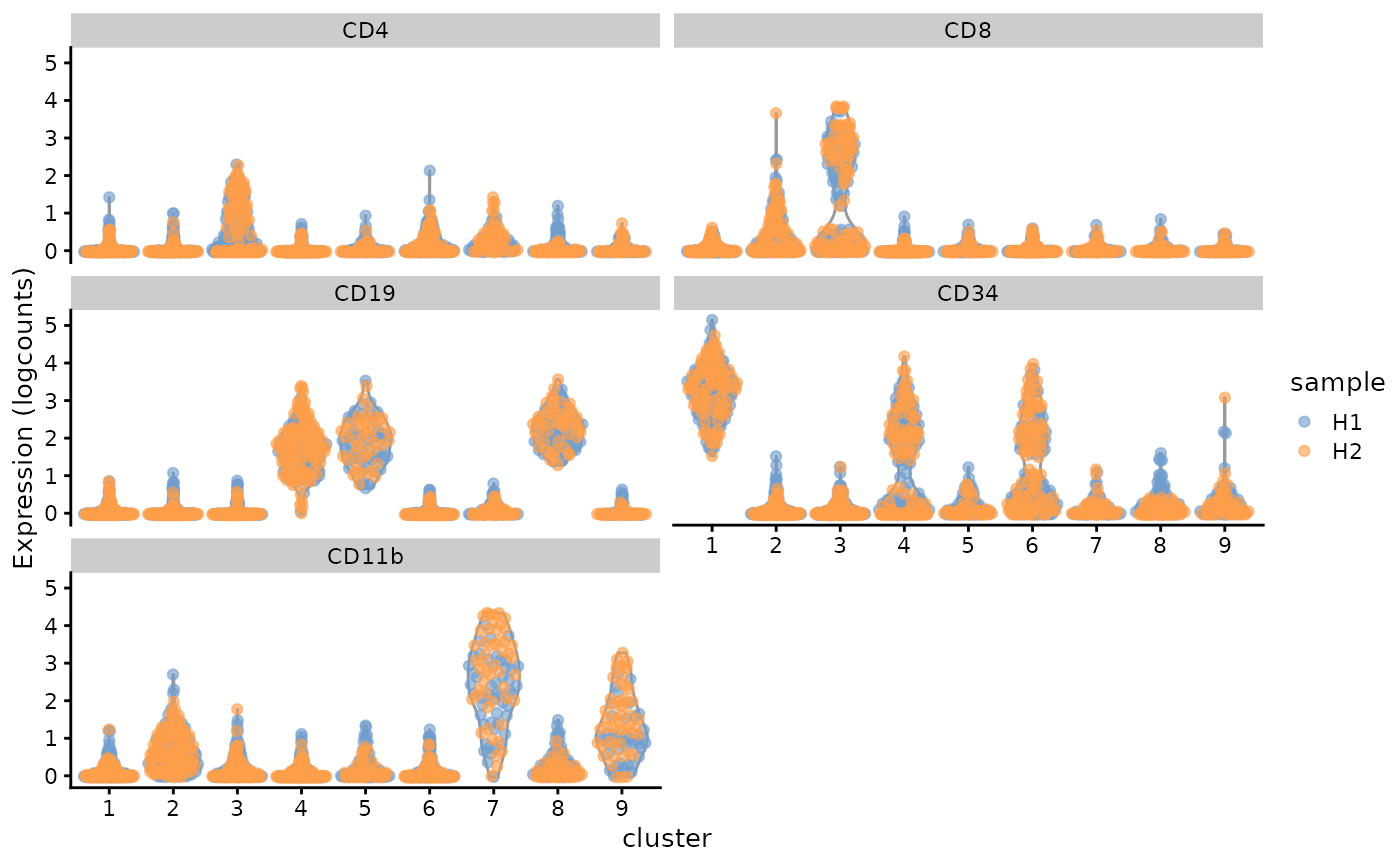
Or violin plot to see the distribution of their marker expressions. Note, the y-axis says “logcounts”, but the data is actually arcsinh transformed, not log transformed.

plotExpression(
    sce, c("CD4", "CD8", "CD19", "CD34", "CD11b"),
    x = "cluster", colour_by = "sample"
)

Session information